In physics, a dipole (from Ancient Greek δίς (dís) 'twice' and πόλος (pólos) 'axis')^[1][2][3] is an electromagnetic phenomenon which occurs in two ways:

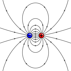
• An electric dipole formed by the separation of the positive and negative electric charges (typically in atomic and molecular systems). Electric dipoles are typically represented by a pair of charges of equal but opposite electric charges separated by a small distance.
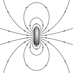
• A magnetic dipole represents a sufficiently small magnet such as those due to atoms, molecules, and electrons. Magnetic dipoles are typically modeled as a loop of constant current.^[4][5]

Dipoles, whether electric or magnetic, can be characterized by their dipole moment, a vector quantity. The electric dipole moment points from the negative charge towards the positive charge and has a magnitude equal to the strength of each charge times the separation between the charges.^{[note 1]} For magnetic dipoles, the magnetic dipole moment points through the loop (according to the right hand grip rule), with a magnitude equal to the current in the loop times the area of the loop.

Electric dipoles produce an electric field and experience forces and torques in an electric field that are proportional to their electric dipole moments. The same is true of magnetic dipoles with magnetic fields. Too, the relations between the electric dipole moment and electric fields are nearly identical to the relations between the magnetic dipole and the magnetic field.

Objects having positive and negative charge with no net charge (such as atoms or molecules) can often be modeled as an electric dipole. For sufficiently large distances (or equivalently sufficiently small objects), the complexities of these object can be ignored so that all of the physics depends on one quantity the electric dipole moment. In this model, the object is represented as two equal but opposite point charges with charge ±q and separated by a distance d. The electric dipole moment has a magnitude 👁 {\displaystyle p=qd}
and is directed from the negative charge to the positive one.

A better definition, accounting for the vector nature of the dipole moment, expresses the electric dipole moment p in vector form 👁 {\displaystyle \mathbf {p} =q\mathbf {d} }
where d is the displacement vector pointing from the negative charge to the positive charge. The electric dipole moment vector p then points in the same direction. With this definition, the dipole direction tends to align itself with an external electric field (which tends to oppose the flux lines of the external field). Note that this sign convention is used in physics, while the opposite sign convention for the dipole, from the positive charge to the negative charge, is used in chemistry.^[6]

A magnetic dipole is a theoretical description of a sufficiently small magnet such as that of an atom or an electron. All magnets can be described as being a magnetic dipole for sufficiently large distances from the magnet. The strength of a magnetic dipole is determined by a single property: its magnetic dipole moment, m. The magnetic dipole model accurately predicts many properties of small magnets such as the magnetic field it produces and how it interacts with other magnetic dipoles, and external magnetic fields.

Two different models can be used to describe a magnetic dipole. The simplest to understand, but least correct, is to imagine the magnet as 2 equal but opposite poles. The magnetic dipole moment, similar to the electric dipole moment, then is the product of the magnetic charge (also known as pole strength) and the vector distance between the charges. This can give correct results in an easy to understand way, but suffers from being incorrect (magnetic poles do not exist as separate entities) and giving incorrect results in certain cases (for example inside of a magnet).

The more correct description of a magnetic dipole is that of a closed loop of electric current that encloses a flat area a. The magnetic moment of this dipole then is the product of its area and it current I. This amperian loop model has the advantage of being physically correct, at least for the part of the magnetic field of an atom due to the motion of the electrons around the nucleus of atoms.

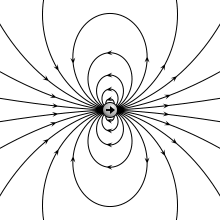
A physical dipole consists of two equal and opposite point charges: in the literal sense, two poles. Its field at large distances (i.e., distances large in comparison to the separation of the poles) depends almost entirely on the dipole moment as defined above. A point (electric) dipole or ideal dipole is the limit obtained by letting the separation tend to 0 while keeping the dipole moment fixed. The field of a point dipole has a particularly simple form, and the order-1 term in the multipole expansion is precisely the point dipole field.

Any finite size charge distribution near the origin can be expressed equivalently as an infinite sum of infinitesimally small charge distributions at the origin with progressively finer angular features. (Something similar happens for finite size current distributions producing magnetic fields.) One advantage of this multipole expansion is that for sufficiently large distances from the origin the first non-zero term of this series dominates. For electric and magnetic fields this term is typically the electric and magnetic dipole respectively.

The first term in the multipole expansion is the monopole. It represents the total charge of the charge distribution and produces spherically symmetric fields (electric field E for the electric dipole or magnetic field B for the magnetic dipole) that decrease as ⁠1/r²⁠. Magnetic monopoles do not exist in nature, therefore they don't contribute to the magnetic field. Electric monopoles (isolated electric charges) exist but do not contribute for the common case of materials with no net electrical charge.

Any configuration of charges or currents has a 'dipole moment' whose field is the best approximation, at large distances, to that of that configuration. The field of a dipole falls off in proportion to ⁠1/r³⁠, as compared to ⁠1/r⁴⁠ for the next (quadrupole) term and higher powers of ⁠1/r⁠ for higher terms.

Although there are no known magnetic monopoles in nature, magnetic dipoles exist in the form of the quantum-mechanical spin associated with particles such as electrons and the 'currents' of electrons around nuclei. A theoretical magnetic point dipole has a magnetic field of the same form as the electric field of an electric point dipole. A very small current-carrying loop is approximately a magnetic point dipole; the magnetic dipole moment of such a loop is the product of the current flowing in the loop and the (vector) area of the loop.

In electromagnetism, the calculation of the electric and magnetic fields are often made simpler by first calculating the scaler and vector potentials, Φ and A respectively.

The electrostatic potential at position r due to an electric dipole at the origin is given by:

👁 {\displaystyle \Phi (\mathbf {r} )={\frac {1}{4\pi \varepsilon _{0}}}\,{\frac {\mathbf {p} \cdot {\hat {\mathbf {r} }}}{r^{2}}},}
where p is the electric dipole moment, and ε₀ is the permittivity of free space. This term appears as the second term in the multipole expansion of an arbitrary electrostatic potential Φ(r). This term will dominate at large distances if there is no net charge (and if p≠0).

The vector potential A at position r of a magnetic dipole moment m at the origin is

👁 {\displaystyle \mathbf {A} (\mathbf {r} )={\frac {\mu _{0}}{4\pi }}{\frac {\mathbf {m} \times {\hat {\mathbf {r} }}}{r^{2}}},}

where μ₀ is the permeability of free space. This term appears as the second term (first non-zero term) in the multipole expansion of an arbitrary vector potential A(r) in terms of the current density J that created it. This term dominates at large distances if m≠0.

The electric field, E, at a location r due to an electric dipole at the origin with electric dipole moment p can be found from the gradient of the electric potential of the dipole defined above:

👁 {\displaystyle \mathbf {E} =-\nabla \Phi ={\frac {1}{4\pi \varepsilon _{0}}}\ {\frac {3(\mathbf {p} \cdot {\hat {\mathbf {r} }}){\hat {\mathbf {r} }}-\mathbf {p} }{r^{3}}}-\delta ^{3}(\mathbf {r} ){\frac {\mathbf {p} }{3\varepsilon _{0}}},}

where ε₀ is the permitivity of free space. The last term in the equation (containing the dirac delta function) only contributes at the origin and in most cases can be ignored.

The magnetic field B at a location r due to a magnetic dipole at the origin with magnetic dipole moment m is the curl of the vector potential A defined above:

👁 {\displaystyle \mathbf {B} =\nabla \times \mathbf {A} ={\frac {\mu _{0}}{4\pi }}\ {\frac {3(\mathbf {m} \cdot {\hat {\mathbf {r} }}){\hat {\mathbf {r} }}-\mathbf {m} }{r^{3}}}+\delta ^{3}(\mathbf {r} ){\frac {2\mu _{0}\mathbf {m} }{3}},}

where μ₀ is the permeability of free space. Similar to the case with the electric field, the last term in the equation (containing the dirac delta function) only contributes at the origin and in most cases can be ignored.

Note that the equation for the magnetic field of a magnetic dipole is almost identical (apart from the term at the origin) to the equivalent equation for the electric field of an electric dipole.

These equations are exactly the field of a point (ideal) dipole, exactly the dipole term in the multipole expansion of an arbitrary field, and approximately the field of any dipole-like configuration at large distances. The field of a real (physical) dipole is continuous everywhere and will be different close to the origin. The delta function represents the strong field pointing in the opposite direction between the point charges for the electric dipole case (and in same direction for magnetic dipole), which is often omitted since one is rarely interested in the field at the dipole's position.

For further discussions about the internal field of dipoles, see^[5][7] or Magnetic moment § Internal magnetic field of a dipole.

The far-field strength, B, of a dipole magnetic field is given by 👁 {\displaystyle B(m,r,\lambda )={\frac {\mu _{0}}{4\pi }}{\frac {m}{r^{3}}}{\sqrt {1+3\sin ^{2}(\lambda )}}\,,}
where

Conversion to cylindrical coordinates is achieved using r² = z² + ρ² and 👁 {\displaystyle \lambda =\arcsin \left({\frac {z}{\sqrt {z^{2}+\rho ^{2}}}}\right)}
where ρ is the perpendicular distance from the z-axis. Then, 👁 {\displaystyle B(\rho ,z)={\frac {\mu _{0}m}{4\pi \left(z^{2}+\rho ^{2}\right)^{\frac {3}{2}}}}{\sqrt {1+{\frac {3z^{2}}{z^{2}+\rho ^{2}}}}}}

Since the direction of an electric field is defined as the direction of the force on a positive charge, electric field lines point away from a positive charge and toward a negative charge.

When placed in a homogeneous electric or magnetic field, equal but opposite forces arise on each side of the dipole creating a torque τ: 👁 {\displaystyle {\boldsymbol {\tau }}=\mathbf {p} \times \mathbf {E} }
for an electric dipole moment p (in coulomb-meters), or 👁 {\displaystyle {\boldsymbol {\tau }}=\mathbf {m} \times \mathbf {B} }
for a magnetic dipole moment m (in ampere-square meters).

The resulting torque will tend to align the dipole with the applied field, which in the case of an electric dipole, yields a potential energy of 👁 {\displaystyle U=-\mathbf {p} \cdot \mathbf {E} .}

The energy of a magnetic dipole is similarly 👁 {\displaystyle U=-\mathbf {m} \cdot \mathbf {B} .}

Many molecules have such dipole moments due to non-uniform distributions of positive and negative charges on the various atoms. Such is the case with polar compounds like hydrogen fluoride (HF), where electron density is shared unequally between atoms. Therefore, a molecule's dipole is an electric dipole with an inherent electric field that should not be confused with a magnetic dipole, which generates a magnetic field.

The physical chemist Peter J. W. Debye was the first scientist to study molecular dipoles extensively, and, as a consequence, dipole moments are measured in the non-SI unit named debye in his honor.

For molecules there are three types of dipoles:

Permanent dipoles

These occur when two atoms in a molecule have substantially different electronegativity : One atom attracts electrons more than another, becoming more negative, while the other atom becomes more positive. A molecule with a permanent dipole moment is called a polar molecule. See Intermolecular force § Dipole–dipole interactions.

Instantaneous dipoles

These occur due to chance when electrons happen to be more concentrated in one place than another in a molecule, creating a temporary dipole. These dipoles are smaller in magnitude than permanent dipoles, but still play a large role in chemistry and biochemistry due to their prevalence. See instantaneous dipole.

Induced dipoles

These can occur when one molecule with a permanent dipole repels another molecule's electrons, inducing a dipole moment in that molecule. A molecule is polarized when it carries an induced dipole. See induced-dipole attraction.

More generally, an induced dipole of any polarizable charge distribution ρ (remember that a molecule has a charge distribution) is caused by an electric field external to ρ. This field may, for instance, originate from an ion or polar molecule in the vicinity of ρ or may be macroscopic (e.g., a molecule between the plates of a charged capacitor). The size of the induced dipole moment is equal to the product of the strength of the external field and the dipole polarizability of ρ.

Dipole moment values can be obtained from measurement of the dielectric constant. Some typical gas phase values given with the unit debye are:^[8]

• carbon dioxide: 0
• carbon monoxide: 0.112 D
• ozone: 0.53 D
• phosgene: 1.17 D
• ammonia: 1.42 D
• water vapor: 1.85 D
• hydrogen cyanide: 2.98 D
• cyanamide: 4.27 D
• potassium bromide: 10.41 D

Potassium bromide (KBr) has one of the highest dipole moments because it is an ionic compound that exists as a molecule in the gas phase.

The overall dipole moment of a molecule may be approximated as a vector sum of bond dipole moments. As a vector sum it depends on the relative orientation of the bonds, so that from the dipole moment information can be deduced about the molecular geometry.

For example, the zero dipole of CO₂ implies that the two C=O bond dipole moments cancel so that the molecule must be linear. For H₂O the O−H bond moments do not cancel because the molecule is bent. For ozone (O₃) which is also a bent molecule, the bond dipole moments are not zero even though the O−O bonds are between similar atoms. This agrees with the Lewis structures for the resonance forms of ozone which show a positive charge on the central oxygen atom.

An example in organic chemistry of the role of geometry in determining dipole moment is the cis and trans isomers of 1,2-dichloroethene. In the cis isomer the two polar C−Cl bonds are on the same side of the C=C double bond and the molecular dipole moment is 1.90 D. In the trans isomer, the dipole moment is zero because the two C−Cl bonds are on opposite sides of the C=C and cancel (and the two bond moments for the much less polar C−H bonds also cancel).

Another example of the role of molecular geometry is boron trifluoride, which has three polar bonds with a difference in electronegativity greater than the traditionally cited threshold of 1.7 for ionic bonding. However, due to the equilateral triangular distribution of the fluoride ions centered on and in the same plane as the boron cation, the symmetry of the molecule results in its dipole moment being zero.

Consider a collection of N particles with charges q_i and position vectors r_i. For instance, this collection may be a molecule consisting of electrons, all with charge −e, and nuclei with charge eZ_i, where Z_i is the atomic number of the i th nucleus. The dipole observable (physical quantity) has the quantum mechanical dipole operator:^{[citation needed]} 👁 {\displaystyle {\mathfrak {p}}=\sum _{i=1}^{N}\,q_{i}\,\mathbf {r} _{i}\,.}

Notice that this definition is valid only for neutral atoms or molecules, i.e. total charge equal to zero. In the ionized case, we have 👁 {\displaystyle {\mathfrak {p}}=\sum _{i=1}^{N}\,q_{i}\,(\mathbf {r} _{i}-\mathbf {r} _{c}),}
where 👁 {\displaystyle \mathbf {r} _{c}}
is the center of mass of the molecule/group of particles.^[9]

A non-degenerate (S-state) atom can have only a zero permanent dipole. This fact follows quantum mechanically from the inversion symmetry of atoms. All 3 components of the dipole operator are antisymmetric under inversion with respect to the nucleus, 👁 {\displaystyle {\mathfrak {I}}\;{\mathfrak {p}}\;{\mathfrak {I}}^{-1}=-{\mathfrak {p}},}
where 👁 {\displaystyle {\mathfrak {p}}}
is the dipole operator and 👁 {\displaystyle {\mathfrak {I}}}
is the inversion operator.

The permanent dipole moment of an atom in a non-degenerate state (see Degenerate energy level) is given as the expectation (average) value of the dipole operator, 👁 {\displaystyle \left\langle {\mathfrak {p}}\right\rangle =\left\langle S\right|{\mathfrak {p}}\left|S\right\rangle ,}
where 👁 {\displaystyle \left|S\right\rangle }
is an S-state, non-degenerate, wavefunction, which is symmetric or anti-symmetric under inversion: 👁 {\displaystyle {\mathfrak {I}}\left|S\right\rangle =\pm \left|S\right\rangle }
. Since the product of the wavefunction (in the ket) and its complex conjugate (in the bra) is always symmetric under inversion and its inverse, 👁 {\displaystyle \left\langle {\mathfrak {p}}\right\rangle =\left\langle {\mathfrak {I}}^{-1}S\right|{\mathfrak {p}}\left|{\mathfrak {I}}^{-1}S\right\rangle =\left\langle S\right|{\mathfrak {I}}\,{\mathfrak {p}}\,{\mathfrak {I}}^{-1}\left|S\right\rangle =-\left\langle {\mathfrak {p}}\right\rangle }
it follows that the expectation value changes sign under inversion. We used here the fact that 👁 {\displaystyle {\mathfrak {I}}}
, being a symmetry operator, is unitary: 👁 {\displaystyle {\mathfrak {I}}^{-1}={\mathfrak {I}}^{*}\,}
and by definition the Hermitian adjoint 👁 {\displaystyle {\mathfrak {I}}^{*}\,}
may be moved from bra to ket and then becomes 👁 {\displaystyle {\mathfrak {I}}^{**}={\mathfrak {I}}\,}
. Since the only quantity that is equal to minus itself is the zero, the expectation value vanishes, 👁 {\displaystyle \left\langle {\mathfrak {p}}\right\rangle =0.}

In the case of open-shell atoms with degenerate energy levels, one could define a dipole moment by the aid of the first-order Stark effect. This gives a non-vanishing dipole (by definition proportional to a non-vanishing first-order Stark shift) only if some of the wavefunctions belonging to the degenerate energies have opposite parity; i.e., have different behavior under inversion. This is a rare occurrence, but happens for the excited H-atom, where 2s and 2p states are "accidentally" degenerate (see article Laplace–Runge–Lenz vector for the origin of this degeneracy) and have opposite parity (2s is even and 2p is odd).

In addition to dipoles in electrostatics, it is also common to consider an electric or magnetic dipole that is oscillating in time. It is an extension, or a more physical next-step, to spherical wave radiation.

In particular, consider a harmonically oscillating electric dipole, with angular frequency ω and a dipole moment p₀ along the ẑ direction of the form 👁 {\displaystyle \mathbf {p} (\mathbf {r} ,t)=\mathbf {p} (\mathbf {r} )e^{-i\omega t}=p_{0}{\hat {\mathbf {z} }}e^{-i\omega t}.}

In vacuum, the exact field produced by this oscillating dipole can be derived using the retarded potential formulation as: 👁 {\displaystyle {\begin{aligned}\mathbf {E} &={\frac {1}{4\pi \varepsilon _{0}}}\left[{\frac {\omega ^{2}}{c^{2}r}}\left({\hat {\mathbf {r} }}\times \mathbf {p} \right)\times {\hat {\mathbf {r} }}+\left({\frac {1}{r^{3}}}-{\frac {i\omega }{cr^{2}}}\right)\left(3{\hat {\mathbf {r} }}\left[{\hat {\mathbf {r} }}\cdot \mathbf {p} \right]-\mathbf {p} \right)\right]e^{i\omega (r/c-t)}\\[1ex]\mathbf {B} &={\frac {\omega ^{2}}{4\pi \varepsilon _{0}c^{3}}}({\hat {\mathbf {r} }}\times \mathbf {p} )\left(1-{\frac {c}{i\omega r}}\right){\frac {e^{i\omega (r/c-t)}}{r}}.\end{aligned}}}

For ⁠rω/c⁠ ≫ 1, the far-field takes the simpler form of a radiating "spherical" wave, but with angular dependence embedded in the cross-product:^[10] 👁 {\displaystyle {\begin{aligned}\mathbf {B} &={\frac {\omega ^{2}}{4\pi \varepsilon _{0}c^{3}}}({\hat {\mathbf {r} }}\times \mathbf {p} ){\frac {e^{i\omega (r/c-t)}}{r}}\\[0.4ex]&={\frac {\omega ^{2}\mu _{0}p_{0}}{4\pi c}}({\hat {\mathbf {r} }}\times {\hat {\mathbf {z} }}){\frac {e^{i\omega (r/c-t)}}{r}}=-{\frac {\omega ^{2}\mu _{0}p_{0}}{4\pi c}}\sin(\theta ){\frac {e^{i\omega (r/c-t)}}{r}}{\hat {\boldsymbol {\phi }}}\\[1ex]\mathbf {E} &=c\mathbf {B} \times {\hat {\mathbf {r} }}\\[0.4ex]&=-{\frac {\omega ^{2}\mu _{0}p_{0}}{4\pi }}\sin(\theta )\left({\hat {\boldsymbol {\phi }}}\times \mathbf {\hat {r}} \right){\frac {e^{i\omega (r/c-t)}}{r}}=-{\frac {\omega ^{2}\mu _{0}p_{0}}{4\pi }}\sin(\theta ){\frac {e^{i\omega (r/c-t)}}{r}}{\hat {\boldsymbol {\theta }}}.\end{aligned}}}

The time-averaged Poynting vector 👁 {\displaystyle \langle \mathbf {S} \rangle ={\frac {\mu _{0}p_{0}^{2}\omega ^{4}}{32\pi ^{2}c}}\,{\frac {\sin ^{2}(\theta )}{r^{2}}}\mathbf {\hat {r}} }
is not distributed isotropically, but concentrated around the directions lying perpendicular to the dipole moment, as a result of the non-spherical electric and magnetic waves. In fact, the spherical harmonic function (sin θ) responsible for such toroidal angular distribution is precisely the l = 1 "p" wave.

The total time-average power radiated by the field can then be derived from the Poynting vector as 👁 {\displaystyle P={\frac {\mu _{0}\omega ^{4}p_{0}^{2}}{12\pi c}}.}

Notice that the dependence of the power on the fourth power of the frequency of the radiation is in accordance with the Rayleigh scattering, and the underlying effects why the sky consists of mainly blue colour.

A circular polarized dipole is described as a superposition of two linear dipoles.

• USGS Geomagnetism Program
• Fields of Force Archived 2010-12-14 at the Wayback Machine: a chapter from an online textbook
• Electric Dipole Potential by Stephen Wolfram and Energy Density of a Magnetic Dipole by Franz Krafft. Wolfram Demonstrations Project.

References

[edit]- ^ δίς, Henry George Liddell, Robert Scott, A Greek-English Lexicon, on Perseus
- ^ πόλος, Henry George Liddell, Robert Scott, A Greek-English Lexicon, on Perseus
- ^ "dipole, n.". Oxford English Dictionary (2nd ed.). Oxford University Press. 1989.
- ^ Brau, Charles A. (2004). Modern Problems in Classical Electrodynamics. Oxford University Press. ISBN 0-19-514665-4.
- ^ a b Griffiths, David J. (1999). Introduction to Electrodynamics (3rd ed.). Prentice Hall. ISBN 0-13-805326-X.
- ^ Peter W. Atkins; Loretta Jones (2016). Chemical principles: the quest for insight (7th ed.). Macmillan Learning. ISBN 978-1-4641-8395-9.
- ^ Jackson, John D. (1999). Classical Electrodynamics, 3rd Ed. Wiley. pp. 148–150. ISBN 978-0-471-30932-1.
- ^ Weast, Robert C. (1984). CRC Handbook of Chemistry and Physics (65th ed.). CRC Press. ISBN 0-8493-0465-2.
- ^ "The Electric Dipole Moment Vector -- Direction, Magnitude, Meaning, et cetera".
- ^ David J. Griffiths, Introduction to Electrodynamics, Prentice Hall, 1999, page 447
External links
[edit]- USGS Geomagnetism Program