👁 Image

👁 Image

In the differential geometry of curves, the evolute of a curve is the locus of all its centers of curvature. That is to say that when the center of curvature of each point on a curve is drawn, the resultant shape will be the evolute of that curve. The evolute of a circle is therefore a single point at its center.^[1] Equivalently, an evolute is the envelope of the normals to a curve.

The evolute of a curve, a surface, or more generally a submanifold, is the caustic of the normal map. Let M be a smooth, regular submanifold in Rⁿ. For each point p in M and each vector v, based at p and normal to M, we associate the point p + v. This defines a Lagrangian map, called the normal map. The caustic of the normal map is the evolute of M.^[2]

Evolutes are closely connected to involutes: A curve is the evolute of any of its involutes.

Apollonius (c. 200 BC) discussed evolutes in Book V of his Conics. However, Huygens is sometimes credited with being the first to study them (1673). Huygens formulated his theory of evolutes sometime around 1659 to help solve the problem of finding the tautochrone curve, which in turn helped him construct an isochronous pendulum. This was because the tautochrone curve is a cycloid, and the cycloid has the unique property that its evolute is also a cycloid. The theory of evolutes, in fact, allowed Huygens to achieve many results that would later be found using calculus.^[3]

If 👁 {\displaystyle {\vec {x}}={\vec {c}}(t),\;t\in [t_{1},t_{2}]}
is the parametric representation of a regular curve in the plane with its curvature nowhere 0 and 👁 {\displaystyle \rho (t)}
its curvature radius and 👁 {\displaystyle {\vec {n}}(t)}
the unit normal pointing to the curvature center, then 👁 {\displaystyle {\vec {E}}(t)={\vec {c}}(t)+\rho (t){\vec {n}}(t)}
describes the evolute of the given curve.

For 👁 {\displaystyle {\vec {c}}(t)=(x(t),y(t))^{\mathsf {T}}}
and 👁 {\displaystyle {\vec {E}}=(X,Y)^{\mathsf {T}}}
one gets 👁 {\displaystyle X(t)=x(t)-{\frac {y'(t){\Big (}x'(t)^{2}+y'(t)^{2}{\Big )}}{x'(t)y''(t)-x''(t)y'(t)}}}
and 👁 {\displaystyle Y(t)=y(t)+{\frac {x'(t){\Big (}x'(t)^{2}+y'(t)^{2}{\Big )}}{x'(t)y''(t)-x''(t)y'(t)}}.}

For a curve 👁 {\displaystyle \Gamma }
expressed implicitly in the form 👁 {\displaystyle f(x,y)=0}
, the Evolute can be determined through a system of equations that relates the original curve to its normal lines. At each point on the curve 👁 {\displaystyle \Gamma }
, the direction of the normal vector is given by:

👁 {\displaystyle \left(-{\frac {f_{y}}{f_{x}}},\,{\frac {xf_{y}-yf_{x}}{f_{x}}}\right)}

where 👁 {\displaystyle f_{x}={\frac {\partial f}{\partial x}}}
and 👁 {\displaystyle f_{y}={\frac {\partial f}{\partial y}}}
. These components describe the direction of the normal vector at each point on the curve.

The Evolute can be obtained by solving the following system (see ^[4] for details):

👁 {\displaystyle {\begin{aligned}0&=f(x,y),\\u&=-{\frac {f_{y}}{f_{x}}},\\v&={\frac {xf_{y}-yf_{x}}{f_{x}}},\end{aligned}}}

where 👁 {\displaystyle u}
and 👁 {\displaystyle v}
represent the components of the normal vector. Eliminating the variables 👁 {\displaystyle x}
and 👁 {\displaystyle y}
from this system yields a single algebraic equation in terms of 👁 {\displaystyle u}
and 👁 {\displaystyle v}
, which defines the evolute of the curve.

👁 Image

In order to derive properties of a regular curve it is advantageous to use the arc length 👁 {\displaystyle s}
of the given curve as its parameter, because of 👁 {\textstyle \left|{\vec {c}}'\right|=1}
and 👁 {\textstyle {\vec {n}}'=-{\vec {c}}'/\rho }
(see Frenet–Serret formulas). Hence the tangent vector of the evolute 👁 {\textstyle {\vec {E}}={\vec {c}}+\rho {\vec {n}}}
is: 👁 {\displaystyle {\vec {E}}'={\vec {c}}'+\rho '{\vec {n}}+\rho {\vec {n}}'=\rho '{\vec {n}}\ .}
From this equation one gets the following properties of the evolute:

• At points with 👁 {\displaystyle \rho '=0}
  the evolute is not regular. That means: at points with maximal or minimal curvature (vertices of the given curve) the evolute has cusps. (See the diagrams of the evolutes of the parabola, the ellipse, the cycloid and the nephroid.)
• For any arc of the evolute that does not include a cusp, the length of the arc equals the difference between the radii of curvature at its endpoints. This fact leads to an easy proof of the Tait–Kneser theorem on nesting of osculating circles.^[5]
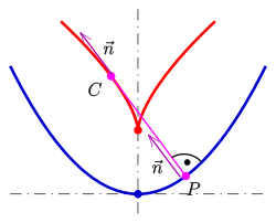
• The normals of the given curve at points of nonzero curvature are tangents to the evolute, and the normals of the curve at points of zero curvature are asymptotes to the evolute. Hence: the evolute is the envelope of the normals of the given curve.
• At sections of the curve with 👁 {\displaystyle \rho '>0}
  or 👁 {\displaystyle \rho '<0}
  the curve is an involute of its evolute. (In the diagram: The blue parabola is an involute of the red semicubic parabola, which is actually the evolute of the blue parabola.)

Proof of the last property:
Let be 👁 {\displaystyle \rho '>0}
at the section of consideration. An involute of the evolute can be described as follows: 👁 {\displaystyle {\vec {C}}_{0}={\vec {E}}-{\frac {{\vec {E}}'}{\left|{\vec {E}}'\right|}}\left(\int _{0}^{s}\left|{\vec {E}}'(w)\right|\mathrm {d} w+l_{0}\right),}
where 👁 {\displaystyle l_{0}}
is a fixed string extension (see Involute of a parameterized curve ).
With 👁 {\displaystyle {\vec {E}}={\vec {c}}+\rho {\vec {n}}\;,\;{\vec {E}}'=\rho '{\vec {n}}}
and 👁 {\displaystyle \rho '>0}
one gets 👁 {\displaystyle {\vec {C}}_{0}={\vec {c}}+\rho {\vec {n}}-{\vec {n}}\left(\int _{0}^{s}\rho '(w)\;\mathrm {d} w\;+l_{0}\right)={\vec {c}}+(\rho (0)-l_{0})\;{\vec {n}}\,.}
That means: For the string extension 👁 {\displaystyle l_{0}=\rho (0)}
the given curve is reproduced.

• Parallel curves have the same evolute.

Proof: A parallel curve with distance 👁 {\displaystyle d}
off the given curve has the parametric representation 👁 {\displaystyle {\vec {c}}_{d}={\vec {c}}+d{\vec {n}}}
and the radius of curvature 👁 {\displaystyle \rho _{d}=\rho -d}
(see parallel curve). Hence the evolute of the parallel curve is 👁 {\displaystyle {\vec {E}}_{d}={\vec {c}}_{d}+\rho _{d}{\vec {n}}={\vec {c}}+d{\vec {n}}+(\rho -d){\vec {n}}={\vec {c}}+\rho {\vec {n}}={\vec {E}}\;.}

From the perspective of singularity theory, evolutes are envelopes of smooth families of lines and can exhibit typical singularities such as cusps. These singularities correspond to critical points of curvature and degeneracies in the family of normals. Evolutes are classic examples of caustics in Lagrangian and symplectic geometry. Ragni Piene, Cordian Riener, and Boris Shapiro conducted a detailed study of the evolutes of plane real-algebraic curves, focusing on their real and complex geometric properties and bounds on the possible singularities that can arise.^[4] They show that for the real setup

• The maximal number of times a real line can intersect the evolute of a real-algebraic curve of degree 👁 {\displaystyle d}
  is at least 👁 {\displaystyle d(d-2)}
  .
• The maximal number of real cusps (vertices) on such an evolute is at least 👁 {\displaystyle d(2d-3)}
  .
• The maximal number of crunodes (real transverse self-intersections) on the evolute and on its dual curve were also studied, with polynomial lower bounds in terms of 👁 {\displaystyle d}
  .^[4]

For the parabola with the parametric representation 👁 {\displaystyle (t,t^{2})}
one gets from the formulae above the equations: 👁 {\displaystyle X=\cdots =-4t^{3}}
👁 {\displaystyle Y=\cdots ={\frac {1}{2}}+3t^{2}\,,}
which describes a semicubic parabola

👁 Image

For the ellipse with the parametric representation 👁 {\displaystyle (a\cos t,b\sin t)}
one gets:^[6] 👁 {\displaystyle X=\cdots ={\frac {a^{2}-b^{2}}{a}}\cos ^{3}t}
👁 {\displaystyle Y=\cdots ={\frac {b^{2}-a^{2}}{b}}\sin ^{3}t\;.}
These are the equations of a non symmetric astroid. Eliminating parameter 👁 {\displaystyle t}
leads to the implicit representation 👁 {\displaystyle (aX)^{\tfrac {2}{3}}+(bY)^{\tfrac {2}{3}}=(a^{2}-b^{2})^{\tfrac {2}{3}}\ .}

👁 Image

For the cycloid with the parametric representation 👁 {\displaystyle (r(t-\sin t),r(1-\cos t))}
the evolute will be:^[7] 👁 {\displaystyle X=\cdots =r(t+\sin t)}
👁 {\displaystyle Y=\cdots =r(\cos t-1)}
which describes a transposed replica of itself.

👁 Image

The evolute of a log-aesthetic curve is another log-aesthetic curve.^[8] One instance of this relation is that the evolute of an Euler spiral is a spiral with Cesàro equation 👁 {\displaystyle \kappa (s)=-s^{-3}}
.^[9]

The evolute

• of a parabola is a semicubic parabola (see above),
• of an ellipse is a non symmetric astroid (see above),
• of a line is an ideal point,
• of a nephroid is a nephroid (half as large, see diagram),
• of an astroid is an astroid (twice as large),
• of a cardioid is a cardioid (one third as large),
• of a circle is its center,
• of a deltoid is a deltoid (three times as large),
• of a cycloid is a congruent cycloid,
• of a logarithmic spiral is the same logarithmic spiral,
• of a tractrix is a catenary.

A curve with a similar definition is the radial of a given curve. For each point on the curve take the vector from the point to the center of curvature and translate it so that it begins at the origin. Then the locus of points at the end of such vectors is called the radial of the curve. The equation for the radial is obtained by removing the x and y terms from the equation of the evolute. This produces 👁 {\displaystyle (X,Y)=\left(-y'{\frac {{x'}^{2}+{y'}^{2}}{x'y''-x''y'}}\;,\;x'{\frac {{x'}^{2}+{y'}^{2}}{x'y''-x''y'}}\right).}

• Weisstein, Eric W. "Evolute". MathWorld.
• Sokolov, D.D. (2001) [1994], "Evolute", Encyclopedia of Mathematics, EMS Press
• Yates, R. C.: A Handbook on Curves and Their Properties, J. W. Edwards (1952), "Evolutes." pp. 86ff
• Evolute on 2d curves.
• Piene, Ragni, Riener, Cordian, Shapiro, Boris. "Return of the Plane Evolute", Annales de l’Institut Fourier*, 75(4), 2025.

Retrieved from "https://en.wikipedia.org/w/index.php?title=Evolute&oldid=1344410398"

References

[edit]- ^ Weisstein, Eric W. "Circle Evolute". MathWorld.
- ^ Arnold, V. I.; Varchenko, A. N.; Gusein-Zade, S. M. (1985). The Classification of Critical Points, Caustics and Wave Fronts: Singularities of Differentiable Maps, Vol 1. Birkhäuser. ISBN 0-8176-3187-9.
- ^ Yoder, Joella G. (2004). Unrolling Time: Christiaan Huygens and the Mathematization of Nature. Cambridge University Press.
- ^ a b c Ragni Piene, Cordian Riener & Boris Shapiro (2025). Return of the Plane Evolute, Annales de l’Institut Fourier, 75(4):1685–1751. doi:10.5802/aif.3703
- ^ Ghys, Étienne; Tabachnikov, Sergei; Timorin, Vladlen (2013). "Osculating curves: around the Tait-Kneser theorem". The Mathematical Intelligencer. 35 (1): 61–66. arXiv:1207.5662. doi:10.1007/s00283-012-9336-6. MR 3041992.
- ^ R.Courant: Vorlesungen über Differential- und Integralrechnung. Band 1, Springer-Verlag, 1955, S. 268.
- ^ Weisstein, Eric W. "Cycloid Evolute". MathWorld.
- ^ Yoshida, N., & Saito, T. (2012). "The Evolutes of Log-Aesthetic Planar Curves and the Drawable Boundaries of the Curve Segments". Computer-Aided Design and Applications. 9 (5): 721–731. doi:10.3722/cadaps.2012.721-731.
{{cite journal}}: CS1 maint: multiple names: authors list (link) - ^ "Evolute of the Euler spiral". Linebender wiki. 2024-03-11.