
👁 File:Window function and frequency response - Rectangular.svg
Size of this PNG preview of this SVG file: 512 × 256 pixels. Other resolutions: 320 × 160 pixels | 640 × 320 pixels | 1,024 × 512 pixels | 1,280 × 640 pixels | 2,560 × 1,280 pixels.
Original file (SVG file, nominally 512 × 256 pixels, file size: 157 KB)
This is a file from the Wikimedia Commons. Information from its description page there is shown below.
Commons is a freely licensed media file repository. You can help.
Commons is a freely licensed media file repository. You can help.
Summary
| Description |
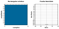
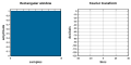
English: Window function and its Fourier transform: Rectangular window |
|||
| Date | ||||
| Source | Own work | |||
| Author | Bob K (original version), Olli Niemitalo, BobQQ | |||
| Permission (Reusing this file) |
I, the copyright holder of this work, hereby publish it under the following license:
|
|||
| Other versions |
The SVG images generated by the enclosed Octave source code replace the older PNG images. See Window function (rectangular).png for example of writing .png files |
|||
| SVG development InfoField | ||||
| Outputs InfoField | The script below generates these SVG images:
This Octave script is not MATLAB-compatible. Things you may need to install to run the script:
For viewing the svg files using "display", you may want to install:
|
|||
| Gnu Octave and Perl Scripts InfoField | Octavegraphics_toolkit gnuplot pkg load signal % Characteristics common to both plots set(0, "DefaultAxesFontName", "Microsoft Sans Serif") set(0, "DefaultTextFontName", "Microsoft Sans Serif") set(0, "DefaultAxesTitleFontWeight", "bold") set(0, "DefaultAxesFontWeight", "bold") set(0, "DefaultAxesFontSize", 20) set(0, "DefaultAxesLineWidth", 3) set(0, "DefaultAxesBox", "on") set(0, "DefaultAxesGridLineStyle", "-") set(0, "DefaultAxesGridColor", [0 0 0]) % black set(0, "DefaultAxesGridAlpha", 0.25) % opaqueness of grid set(0, "DefaultAxesLayer", "bottom") % grid not visible where overlapped by graph %======================================================================== functionplotWindow (w, wname, wfilename = "", wspecifier = "", wfilespecifier = "") close % If there is a previous screen image, remove it. M = 32; % Fourier transform size as multiple of window length Q = 512; % Number of samples in time domain plot P = 40; % Maximum bin index drawn dr = 130; % (dynamic range) Maximum attenuation (dB) drawn in frequency domain plot L = length(w); B = L*sum(w.^2)/sum(w)^2; % noise bandwidth (bins) n = [0 : 1/Q : 1]; w2 = interp1 ([0 : 1/(L-1) : 1], w, n); if (M/L < Q) Q = M/L; endif figure("position", [1 1 1200 600]) % width = 2×height, because there are 2 plots % Plot the window function subplot(1,2,1) area(n,w2,"FaceColor", [0 0.4 0.6], "edgecolor", [0 0 0], "linewidth", 1) g_x = [0 : 1/8 : 1]; % user defined grid X [start:spaces:end] g_y = [0 : 0.1 : 1]; set(gca,"XTick", g_x) set(gca,"YTick", g_y) % Special y-scale if filename includes "flat top" if(index(wname, "flat top")) ylimits = [-0.1 1.05]; else ylimits = [0 1.05]; endif ylim(ylimits) ylabel("amplitude","FontSize",28) set(gca,"XTickLabel",[" 0"; " "; " "; " "; " "; " "; " "; " "; " N"]) grid("on") xlabel("samples","FontSize",28) #{ % This is a disabled work-around for an Octave bug, if you don't want to run the perl post-processor. text(-.18, .4,"amplitude","rotation",90, "Fontsize", 28); text(1.15, .4,"decibels", "rotation",90, "Fontsize", 28); #} %Construct a title from input arguments. %The default interpreter is "tex", which can render subscripts and the following Greek character codes: % \alpha \beta \gamma \delta \epsilon \zeta \eta \theta \vartheta \iota \kappa \lambda \mu \nu \xi \o % \pi \varpi \rho \sigma \varsigma \tau \upsilon \phi \chi \psi \omega. % if (strcmp (wspecifier, "")) title(cstrcat(wname," window"), "FontSize", 28) elseif (length(strfind (wspecifier, "&#")) == 0 ) title(cstrcat(wname,' window (', wspecifier, ')'), "FontSize", 28) else % The specifiers '\sigma_t' and '\mu' work correctly in the output file, but not in subsequent thumbnails. % So UNICODE substitutes are used. The tex interpreter would remove the & character, needed by the Perl script. title(cstrcat(wname,' window (', wspecifier, ')'), "interpreter", "none", "FontSize", 28) endif ax1 = gca; % Compute spectal leakage distribution H = abs(fft([w zeros(1,(M-1)*L)])); H = fftshift(H); H = H/max(H); H = 20*log10(H); H = max(-dr,H); n = ([1:M*L]-1-M*L/2)/M; k2 = [-P : 1/M : P]; H2 = interp1 (n, H, k2); % Plot the leakage distribution subplot(1,2,2) h = stem(k2,H2,"-"); set(h,"BaseValue",-dr) xlim([-P P]) ylim([-dr 6]) set(gca,"YTick", [0 : -10 : -dr]) set(findobj("Type","line"), "Marker", "none", "Color", [0.8710 0.49 0]) grid("on") set(findobj("Type","gridline"), "Color", [.871 .49 0]) ylabel("decibels","FontSize",28) xlabel("bins","FontSize",28) title("Fourier transform","FontSize",28) text(-5, -126, ['B = ' num2str(B,'%5.3f')],"FontWeight","bold","FontSize",14) ax2 = gca; % Configure the plots so that they look right after the Perl post-processor. % These are empirical values (trial & error). % Note: Would move labels and title closer to axes, if I could figure out how to do it. x1 = .08; % left margin for y-axis labels x2 = .02; % right margin y1 = .14; % bottom margin for x-axis labels y2 = .14; % top margin for title ws = .13; % whitespace between plots width = (1-x1-x2-ws)/2; height = 1-y1-y2; set(ax1,"Position", [x1 y1 width height]) % [left bottom width height] set(ax2,"Position", [1-width-x2 y1 width height]) %Construct a filename from input arguments. if (strcmp (wfilename, "")) wfilename = wname; endif if (strcmp (wfilespecifier, "")) wfilespecifier = wspecifier; endif if (strcmp (wfilespecifier, "")) savetoname = cstrcat("Window function and frequency response - ", wfilename, ".svg"); else savetoname = cstrcat("Window function and frequency response - ", wfilename, " (", wfilespecifier, ").svg"); endif print(savetoname, "-dsvg", "-S1200,600") % close % Relocated to the top of the function endfunction %======================================================================== global N L % Generate odd-length, symmetric windows N = 2^16; % Large value ensures most accurate value of B n = 0:N; L = length(n); % Window length %======================================================================== w = ones(1,L); plotWindow(w, "Rectangular") %======================================================================== w = 1 - abs(n-N/2)/(L/2); plotWindow(w, "Triangular") % Indistinguishable from Triangular for large N % w = 1 - abs(n-N/2)/(N/2); % plotWindow(w, "Bartlett") %======================================================================== w = parzenwin(L).'; plotWindow(w, "Parzen"); %======================================================================== w = 1-((n-N/2)/(N/2)).^2; plotWindow(w, "Welch"); %======================================================================== w = sin(pi*n/N); plotWindow(w, "Sine") %======================================================================== w = 0.5 - 0.5*cos(2*pi*n/N); plotWindow(w, "Hann") %======================================================================== w = 0.53836 - 0.46164*cos(2*pi*n/N); plotWindow(w, "Hamming", "Hamming", 'a_0 = 0.53836', "alpha = 0.53836") %======================================================================== w = 0.42 - 0.5*cos(2*pi*n/N) + 0.08*cos(4*pi*n/N); plotWindow(w, "Blackman") %======================================================================== w = 0.355768 - 0.487396*cos(2*pi*n/N) + 0.144232*cos(4*pi*n/N) -0.012604*cos(6*pi*n/N); plotWindow(w, "Nuttall", "Nuttall", "continuous first derivative") %======================================================================== w = 0.3635819 - 0.4891775*cos(2*pi*n/N) + 0.1365995*cos(4*pi*n/N) -0.0106411*cos(6*pi*n/N); plotWindow(w, "Blackman-Nuttall", "Blackman-Nuttall") %======================================================================== w = 0.35875 - 0.48829*cos(2*pi*n/N) + 0.14128*cos(4*pi*n/N) -0.01168*cos(6*pi*n/N); plotWindow(w, "Blackman-Harris", "Blackman-Harris") %======================================================================== % Matlab coefficients a = [0.21557895 0.41663158 0.277263158 0.083578947 0.006947368]; % Stanford Research Systems (SRS) coefficients % a = [1 1.93 1.29 0.388 0.028]; % a = a / sum(a); w = a(1) - a(2)*cos(2*pi*n/N) + a(3)*cos(4*pi*n/N) -a(4)*cos(6*pi*n/N) +a(5)*cos(8*pi*n/N); plotWindow(w, "flat top") %======================================================================== % The version using \sigma no longer renders correct thumbnail previews. % Ollie's older version using σ seems to solve that problem. sigma = 0.4; w = exp(-0.5*( (n-N/2)/(sigma*N/2) ).^2); % plotWindow(w, "Gaussian", "Gaussian", '\sigma = 0.4', "sigma = 0.4") plotWindow(w, "Gaussian", "Gaussian", "σ = 0.4", "sigma = 0.4") %======================================================================== % Confined Gaussian global T P abar target_stnorm N = 512; % Reduce N to avoid excessive computation time n = 0:N; L = length(n); % Window length target_stnorm = 0.1; function[g,sigma_w,sigma_t]=CGWn(alpha, M) % determine eigenvectors of M(alpha) global L P T opts.maxit = 10000; if(M ~= L) [g,lambda] = eigs(P + alpha*T, M, 'sa', opts); else [g,lambda] = eig(P + alpha*T); end sigma_t = sqrt(diag((g'*T*g) / (g'*g))); sigma_w = sqrt(diag((g'*P*g) / (g'*g))); end function[h1]=helperCGW(anorm) global L abar target_stnorm [~,~,sigma_t] = CGWn(anorm*abar,1); h1 = sigma_t - target_stnorm * L; end % define alphabar, and matrices T and P T = zeros(L,L); P = zeros(L,L); for m=1:L T(m,m) = (m - (L+1)/2)^2; for l=1:L if m ~= l P(m,l) = 2*(-1)^(m-l)/(m-l)^2; else P(m,l) = pi^2/3; end end end abar = (10/L)^4/4; [anorm, aval] = fzero(@helperCGW, 0.1/target_stnorm); [CGWg, CGWsigma_w, CGWsigma_t] = CGWn(anorm*abar,1); sigma_t = CGWsigma_t/L % Confirm sigma_t w = CGWg * sign(mean(CGWg)); w = w'/max(w); % \sigma_t works correctly in actual file, but not in thumbnail versions. % plotWindow(w, "Confined Gaussian", "Confined Gaussian", '\sigma_t = 0.1', "sigma_t = 0.1"); plotWindow(w, "Confined Gaussian", "Confined Gaussian", "σₜ = 0.1", "sigma_t = 0.1"); N = 2^16; % restore original N n = 0:N; L = length(n); % Window length %======================================================================== global denominator; sigma = 0.1; denominator = (2*L*sigma).^2; function[gaussout]=gauss(x) global N denominator gaussout = exp(- (x-N/2).^2 ./ denominator); end w = gauss(n) - gauss(-1/2).*(gauss(n+L) + gauss(n-L))./(gauss(-1/2 + L) + gauss(-1/2 - L)); % \sigma_t works correctly in actual file, but not in thumbnail versions % plotWindow(w, "App. conf. Gaussian", "Approximate confined Gaussian", '\sigma_t = 0.1', "sigma_t = 0.1"); plotWindow(w, "App. conf. Gaussian", "Approximate confined Gaussian", "σₜ = 0.1", "sigma_t = 0.1"); %======================================================================== alpha = 0.5; a = alpha*N/2; w = ones(1,L); m = 0 : a; if( max(m) == a ) m = m(1:end-1); endif M = length(m); w(1:M) = 0.5*(1-cos(pi*m/a)); w(L:-1:L-M+1) = w(1:M); % plotWindow(w, "Tukey", "Tukey", '\alpha = 0.5', "alpha = 0.5") plotWindow(w, "Tukey", "Tukey", "α = 0.5", "alpha = 0.5") %======================================================================== epsilon = 0.1; a = N*epsilon; w = ones(1,L); m = 0 : a; if( max(m) == a ) m = m(1:end-1); endif % Divide by 0 is handled by Octave. Results in w(1) = 0. z_exp = a./m - a./(a-m); M = length(m); w(1:M) = 1 ./ (exp(z_exp) + 1); w(L:-1:L-M+1) = w(1:M); #{ % The original method is harder to understand: t_cut = N/2 - a; T_in = abs(n - N/2); z_exp = (t_cut - N/2) ./ (T_in - t_cut)... + (t_cut - N/2) ./ (T_in - N/2); % The numerator forces sigma = 0 at n = 0: sigma = (T_in < N/2) ./ (exp(z_exp) + 1); % Either the 1st term or the 2nd term is 0, depending on n: w = 1 * (T_in <= t_cut) + sigma .* (T_in > t_cut); #} % plotWindow(w, "Planck-taper", "Planck-taper", '\epsilon = 0.1', "epsilon = 0.1") plotWindow(w, "Planck-taper", "Planck-taper", "ε = 0.1", "epsilon = 0.1") %======================================================================== N = 2^12; % Reduce N to avoid excess memory requirement n = 0:N; L = length(n); % Window length alpha = 2; s = sin(alpha*2*pi/L*[1:N])./[1:N]; c0 = [alpha*2*pi/L,s]; A = toeplitz(c0); [V,evals] = eigs(A, 1); [emax,imax] = max(abs(diag(evals))); w = abs(V(:,imax)); w = w.'; w = w / max(w); % plotWindow(w, "DPSS", "DPSS", '\alpha = 2', "alpha = 2") plotWindow(w, "DPSS", "DPSS", "α = 2", "alpha = 2") %======================================================================== alpha = 3; s = sin(alpha*2*pi/L*[1:N])./[1:N]; c0 = [alpha*2*pi/L,s]; A = toeplitz(c0); [V,evals] = eigs(A, 1); [emax,imax] = max(abs(diag(evals))); w = abs(V(:,imax)); w = w.'; w = w / max(w); % plotWindow(w, "DPSS", "DPSS", '\alpha = 3', "alpha = 3") plotWindow(w, "DPSS", "DPSS", "α = 3", "alpha = 3") N = 2^16; % Restore original N n = 0:N; L = length(n); % Window length %======================================================================== alpha = 2; w = besseli(0,pi*alpha*sqrt(1-(2*n/N -1).^2))/besseli(0,pi*alpha); % plotWindow(w, "Kaiser", "Kaiser", '\alpha = 2', "alpha = 2") plotWindow(w, "Kaiser", "Kaiser", "α = 2", "alpha = 2") %======================================================================== alpha = 3; w = besseli(0,pi*alpha*sqrt(1-(2*n/N -1).^2))/besseli(0,pi*alpha); % plotWindow(w, "Kaiser", "Kaiser", '\alpha = 3', "alpha = 3") plotWindow(w, "Kaiser", "Kaiser", "α = 3", "alpha = 3") %======================================================================== alpha = 5; % Attenuation in 20 dB units w = chebwin(L, alpha * 20).'; % plotWindow(w, "Dolph-Chebyshev", "Dolph-Chebyshev", '\alpha = 5', "alpha = 5") plotWindow(w, "Dolph–Chebyshev", "Dolph-Chebyshev", "α = 5", "alpha = 5") %======================================================================== w = ultrwin(L, -.5, 100, 'a')'; % \mu works correctly in actual file, but not in thumbnail versions % plotWindow(w, "Ultraspherical", "Ultraspherical", '\mu = -0.5', "mu = -0.5") plotWindow(w, "Ultraspherical", "Ultraspherical", "μ = -0.5", "mu = -0.5") %======================================================================== tau = (L/2); w = exp(-abs(n-N/2)/tau); % plotWindow(w, "Exponential", "Exponential", '\tau = N/2', "half window decay") plotWindow(w, "Exponential", "Exponential", "τ = N/2", "half window decay") %======================================================================== tau = (L/2)/(60/8.69); w = exp(-abs(n-N/2)/tau); % plotWindow(w, "Exponential", "Exponential", '\tau = (N/2)/(60/8.69)', "60dB decay") plotWindow(w, "Exponential", "Exponential", "τ = (N/2)/(60/8.69)", "60dB decay") %======================================================================== w = 0.62 -0.48*abs(n/N -0.5) -0.38*cos(2*pi*n/N); plotWindow(w, "Bartlett-Hann", "Bartlett-Hann") %======================================================================== alpha = 4.45; epsilon = 0.1; t_cut = N * (0.5 - epsilon); t_in = n - N/2; T_in = abs(t_in); z_exp = ((t_cut - N/2) ./ (T_in - t_cut) + (t_cut - N/2) ./ (T_in - N/2)); sigma = (T_in < N/2) ./ (exp(z_exp) + 1); w = (1 * (T_in <= t_cut) + sigma .* (T_in > t_cut)) .* besseli(0, pi*alpha * sqrt(1 - (2 * t_in / N).^2)) / besseli(0, pi*alpha); % plotWindow(w, "Planck-Bessel", "Planck-Bessel", '\epsilon = 0.1, \alpha = 4.45', "epsilon = 0.1, alpha = 4.45") plotWindow(w, "Planck–Bessel", "Planck-Bessel", "ε = 0.1, α = 4.45", "epsilon = 0.1, alpha = 4.45") %======================================================================== alpha = 2; w = 0.5*(1 - cos(2*pi*n/N)).*exp( -alpha*abs(N-2*n)/N ); % plotWindow(w, "Hann-Poisson", "Hann-Poisson", '\alpha = 2', "alpha = 2") plotWindow(w, "Hann–Poisson", "Hann-Poisson", "α = 2", "alpha = 2") %======================================================================== w = sinc(2*n/N - 1); plotWindow(w, "Lanczos") %======================================================================== % optimized Nutall ak = [-1.9501232504232442 1.7516390954528638 -0.9651321809782892 0.3629219021312954 -0.0943163918335154 ... 0.0140434805881681 0.0006383045745587 -0.0009075461792061 0.0002000671118688 -0.0000161042445001]; n = -N/2:N/2; n = n/std(n); w = 1; for k = 1 : length(ak) % This is an array addition, which expands the dimension of w[] as needed, and the value "1" is replicated. w = w + ak(k)*(n.^(2*k)); endfor w = w/max(w); plotWindow(w, "GAP optimized Nuttall")
Perl code#!/usr/bin/perl opendir(DIR,'.')ordie$!;## open the current directory , if error exit while($file=readdir(DIR)){## read all the file names in the current directory $ext=substr($file,length($file)-4);## get the last 4 letters of the file name if($exteq'.svg'){## if the file extension is '.svg' print("$file\n");## print file name ($pre,$name)=split(" - ",substr($file,0,length($file)-4));## split the filename in 2 @lines=();## dummy up an array open(INPUTFILE,"<",$file)ordie$!;## open up the file for reading while($line=<INPUTFILE>){## loop through all the lines in the file $line=~s/&/&/g;## replace "&" with "&" , get rid of semicolon if($lineeq"<title>Gnuplot</title>\n"){## if line is EXACTLY equal to "<.....>\n" then $line='<title>Window function and its Fourier transform – '.$name."</title>"."\n";## set the line to a new value, – - is unicode for a dash ## the .$name. concatenates the strings together }## end if @lines[0+@lines]=$line;## append to the output array the value of the modified line }## end loop close(INPUTFILE);## close the input file open(OUTPUTFILE,">",$file)ordie$!;## open the output file for($t=0;$t<@lines;$t++){## loop through the output array, printing out each line print(OUTPUTFILE$lines[$t]); }## end loop close(OUTPUTFILE);## close the output file }## end if }## end loop closedir(DIR);## close the directory |
.png)
.png#Octave_commands)
.svg)
.svg)
.svg)
.svg)
.svg)
.svg)
.svg)
.svg)
.svg)
.svg)
.svg)
.svg)
.svg)
.svg)
.svg)
.svg)
.svg)
.svg)
.svg)
.svg)
File history
Click on a date/time to view the file as it appeared at that time.
| Date/Time | Thumbnail | Dimensions | User | Comment | |
|---|---|---|---|---|---|
| current | 17:48, 20 November 2019 | 👁 Thumbnail for version as of 17:48, 20 November 2019 | 512 × 256 (157 KB) | Bob K | Display parameter B on frequency distribution |
| 22:54, 5 April 2019 | 👁 Thumbnail for version as of 22:54, 5 April 2019 | 512 × 256 (156 KB) | Bob K | Change xticks label from N-1 to N, because of changes to article [Window function] | |
| 20:27, 16 February 2013 | 👁 Thumbnail for version as of 20:27, 16 February 2013 | 512 × 256 (131 KB) | Olli Niemitalo | Frequency response --> Fourier transform | |
| 09:18, 13 February 2013 | 👁 Thumbnail for version as of 09:18, 13 February 2013 | 512 × 256 (131 KB) | Olli Niemitalo | Font, dB range | |
| 03:01, 13 February 2013 | 👁 Thumbnail for version as of 03:01, 13 February 2013 | 512 × 256 (131 KB) | Olli Niemitalo | User created page with UploadWizard |
File usage
The following page uses this file:
Global file usage
The following other wikis use this file:
- Usage on ko.wikipedia.org
- Usage on pl.wikipedia.org
Metadata
This file contains additional information, probably added from the digital camera or scanner used to create or digitize it.
If the file has been modified from its original state, some details may not fully reflect the modified file.
| Short title | Window function and its Fourier transform – Rectangular |
|---|---|
| Image title | Produced by GNUPLOT 5.2 patchlevel 6 |
| Width | 100% |
| Height | 100% |