This article examines different notations for the composition of permutations with each other and with vectors.

Permutations are bijections from a set to itself, and the set does not need to have an order.
They can also be described as operations that move things from one set of places to another set of places — which is the natural mental image when the permutation is, e.g., a rotation of a cube.
In the end it does not matter what kind of mental image is used to understand what a permutation is or does, as long as there is no ambiguity about what result a formula will yield.
When a permutation 👁 {\displaystyle \pi }
is interpreted as moving objects from starting places to other places, there are two ways to describe it.

The usual way is as an active permutation or map or substitution:

👁 {\displaystyle \pi }
moves an object from place 👁 {\displaystyle i}
to place 👁 {\displaystyle \pi (i)}
. In an arrow diagram, the one-line notation denotes where the arrows go.

In this case, the result of applying 👁 {\displaystyle \pi }
to a vector 👁 {\displaystyle (x_{1},\dots ,x_{n})}
is 👁 {\displaystyle (x_{\pi ^{-1}(1)},\dots ,x_{\pi ^{-1}(n)})}
.

👁 {\displaystyle \pi }
may also be represented as the result of applying it to the natural order. This is called a passive permutation^[1] or (re)arrangement or ordering:

👁 {\displaystyle \pi }
replaces an object in position 👁 {\displaystyle i}
by that in position 👁 {\displaystyle \pi (i)}
. In an arrow diagram, the one-line notation denotes where the arrows come from.

In this case the result of applying 👁 {\displaystyle \pi }
to a vector 👁 {\displaystyle (x_{1},\dots ,x_{n})}
is 👁 {\displaystyle (x_{\pi (1)},\dots ,x_{\pi (n)})}
.

Confusing these two interpretations will lead to confusing permutations with their inverses.
Active and passive transformations seem to be a related concept.

Composition of permutations is associative, but not commutative.

With prefix notation or left action, 👁 {\displaystyle \pi \sigma (x)=\pi {\bigl (}\sigma (x){\bigr )}}
.

👁 {\displaystyle \pi \sigma }
can be thought of as 👁 {\displaystyle \pi ~{\scriptstyle after}~\sigma }
, and 👁 {\displaystyle \pi x}
as 👁 {\displaystyle \pi ~{\scriptstyle of}~x}

This notation corresponds to the usual way of writing function compositions.

With postfix notation or right action, 👁 {\displaystyle \pi \sigma (x)=x\pi \sigma =\sigma {\bigl (}\pi (x){\bigr )}}
.

👁 {\displaystyle \pi \sigma }
can be thought of as 👁 {\displaystyle \pi ~{\scriptstyle before}~\sigma }
, and 👁 {\displaystyle x\pi }
as (image of) 👁 {\displaystyle x~{\scriptstyle under}~\pi }
.

This notation is common in group theory.

(In the Python examples in this article (P*Q)(2) = 2^P^Q = Q(P(2)). The result is R(2) = 4).

In its graphics this article shows all possible interpretations, including the passive ones.
To avoid confusion, however, the accompanying calculations use only active right notation, which is the notation used by SymPy and Wolfram.

👁 {\displaystyle \alpha ={\begin{pmatrix}1&2&3\\3&1&2\end{pmatrix}},~\beta ={\begin{pmatrix}1&2&3\\2&1&3\end{pmatrix}},~v=(v_{1},v_{2},v_{3}),~~~~~~~~~~~\alpha ^{-1}={\begin{pmatrix}1&2&3\\2&3&1\end{pmatrix}}}

If permuting 👁 {\displaystyle v}
by 👁 {\displaystyle \alpha }
gives 👁 {\displaystyle (v_{\alpha ^{-1}(1)},v_{\alpha ^{-1}(2)},v_{\alpha ^{-1}(3)})=(v_{2},v_{3},v_{1})}
the permutation is active.

If permuting 👁 {\displaystyle v}
by 👁 {\displaystyle \alpha }
gives 👁 {\displaystyle (v_{\alpha (1)},v_{\alpha (2)},v_{\alpha (3)})=(v_{3},v_{1},v_{2})}
the permutation is passive.

Passive left should be seen as a misunderstanding of active right, and passive right should be seen as a misunderstanding of active left. ^*

*   (Unless permuting a vector proofs otherwise.)

Permutations can be combined with

• other permutations (boxes 1 to 11)
• vectors of the same length with arbitrary elements (green boxes 12 and 16)
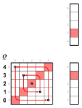
• vectors of arbitrary length with elements from the same range,
  i.e., maps with the same codomain as the permutation, but bijectivity is not required (blue boxes 14 and 15)
• scalars from the same range (red boxes 13 and 17, compare blue box 14)

The variables used in the main examples are

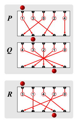
• the permutations 👁 {\displaystyle P={\begin{pmatrix}0&1&2&3&4\\1&3&0&2&4\end{pmatrix}}=(0132)}
  and 👁 {\displaystyle Q={\begin{pmatrix}0&1&2&3&4\\4&3&2&1&0\end{pmatrix}}=(04)(13)}
  
• the vector 👁 {\displaystyle V=(V_{0},\dots ,V_{4})}
  (in the graphics simply 👁 {\displaystyle 0\dots 4}
  )
• the vector 👁 {\displaystyle E=(0,0,4,2,3,2)}
  

In the Wolfram calculations, the 1-based equivalents are used.

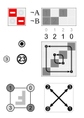
Permutations of four elements are identified by their index numbers in RevCoLex order, i.e., as the 👁 {\displaystyle n}
-th finite permutation.
👁 {\displaystyle P=(0132)}
is denoted 👁 {\displaystyle {\mathit {10}}}
where it appears among other permutations of only four elements. (See box 19, compare with box 1.)
(Equivalents for the permutations of five elements would be 👁 {\displaystyle Q={\mathit {119}}}
, 👁 {\displaystyle R={\mathit {109}}}
and 👁 {\displaystyle S={\mathit {83}}}
^[2], but only the letters are used.)

from sympy.combinatorics import Permutation

def before(positions, sequence):
 return [sequence[i] for i in positions]

def inv(perm):
 length = len(perm)
 if sorted(perm) != list(range(length)):
 print('Inverse not possible!')
 else:
 inverse = [0] * length
 for key, val in enumerate(perm):
 inverse[val] = key
 return inverse

p = [1, 3, 0, 2, 4]
q = [4, 3, 2, 1, 0]
r = before(p, q)

P = Permutation(p)
Q = Permutation(q)
R = P * Q

v = ['0', '1', '2', '3', '4']
e = [0, 0, 4, 2, 3, 2]

p = {2,4,1,3,5}
q = {5,4,3,2,1}
v = {v1,v2,v3,v4,v5}
e = {1,1,5,3,4,3}

A simple rule to avoid passive permutations: If the rows of a permutation matrix are labelled, the cycles must go clockwise (AR). If the columns are labelled, the cycles must go anticlockwise (AL).

The following examples show with arrow diagrams what the composed permutations actually do, and how this can be interpreted as a product in two different ways, corresponding to two different matrix multiplications.

The two arrangements of matrices are symmetric to each other, including the direction of the arrows in the matrices.
In other terms: The matrix image on the left and on the right show exactly the same thing in a different way.
The arrows in both arrangements of matrices are the same as in the arrow diagram to their left.

In prefix notation (left action) 👁 {\displaystyle \alpha \cdot \beta }
means 👁 {\displaystyle \alpha ~{\scriptstyle after}~\beta }
. In postfix notation (right action) 👁 {\displaystyle \beta \cdot \alpha }
means 👁 {\displaystyle \beta ~{\scriptstyle before}~\alpha }
.
Obviously 👁 {\displaystyle \alpha ~{\scriptstyle after}~\beta }
and 👁 {\displaystyle \beta ~{\scriptstyle before}~\alpha }
are just different ways to say the same thing.

>>> Permutation.print_cyclic = True

>>> P
Permutation(4)(0, 1, 3, 2)
>>> Q
Permutation(0, 4)(1, 3)

>>> ~P
Permutation(4)(0, 2, 3, 1)
>>> ~Q
Permutation(0, 4)(1, 3)

>>> ~Q * ~P
Permutation(0, 4, 2, 3)
>>> P * Q
Permutation(0, 3, 2, 4)
>>> Q * P
Permutation(0, 4, 1, 2)

>>> Permutation.print_cyclic = False

>>> P
Permutation[1, 3, 0, 2, 4]
>>> Q
Permutation[4, 3, 2, 1, 0]

>>> ~P
Permutation[2, 0, 3, 1, 4]
>>> ~Q
Permutation[4, 3, 2, 1, 0]

>>> ~Q * ~P
Permutation[4, 1, 3, 0, 2]
>>> P * Q
Permutation[3, 1, 4, 2, 0]
>>> Q * P
Permutation[4, 2, 0, 3, 1]

 
 
>>> p
[1, 3, 0, 2, 4]
>>> q
[4, 3, 2, 1, 0]

>>> inv(p)
[2, 0, 3, 1, 4]
>>> inv(q)
[4, 3, 2, 1, 0]

>>> before(inv(q), inv(p))
[4, 1, 3, 0, 2]
>>> before(p, q)
[3, 1, 4, 2, 0]
>>> before(q, p)
[4, 2, 0, 3, 1]

I: p
O: {2,4,1,3,5}
I: q
O: {5,4,3,2,1}

I: PermutationCycles[p]
O: Cycles[{{1,2,4,3}}]
I: PermutationCycles[q]
O: Cycles[{{1,5},{2,4}}]

I: PermutationProduct[InversePermutation[q], InversePermutation[p]] (* R^-1 *)
O: {5,2,4,1,3}
I: PermutationProduct[p, q] (* R *)
O: {4,2,5,3,1}
I: PermutationProduct[q, p] (* S *)
O: {5,3,1,4,2}

>>> x = before(inv(p), v)
>>> x
['2', '0', '3', '1', '4']

>>> before(inv(q), x) # Y
['4', '1', '3', '0', '2']

>>> before(inv(r), v) # Y
['4', '1', '3', '0', '2']

 
I: x = Permute[v, p]
O: {v3,v1,v4,v2,v5}

I: Permute[x, q] (* Y *)
O: {v5,v2,v4,v1,v3}

I: Permute[v, r] (* Y *)
O: {v5,v2,v4,v1,v3}

>>> before([0], p)
[1]

>>> before([1], q)
[3]

>>> before([0], r)
[3]

I: PermutationReplace[1, p]
O: 2

I: PermutationReplace[2, q]
O: 4

I: PermutationReplace[1, r]
O: 4

>>> f = before(e, p)
>>> f
[1, 1, 4, 0, 2, 0]

>>> before(f, q) # G
[3, 3, 0, 4, 2, 4]

>>> before(e, r) # G
[3, 3, 0, 4, 2, 4]

 
I: f = PermutationReplace[e, p]
O: {2,2,5,1,3,1}

I: PermutationReplace[f, q] (* G *)
O: {4,4,1,5,3,5}

I: PermutationReplace[e, r] (* G *)
O: {4,4,1,5,3,5}

>>> a = before(q, v)
>>> a
['4', '3', '2', '1', '0']

>>> before(p, a) # B
['3', '1', '4', '2', '0']

>>> before(r, v) # B
['3', '1', '4', '2', '0']

 
I: a = Permute[v, InversePermutation[q]]
O: {v5,v4,v3,v2,v1}

I: Permute[a, InversePermutation[p]] (* B *)
O: {v4,v2,v5,v3,v1}

I: Permute[v, InversePermutation[r]] (* B *)
O: {v4,v2,v5,v3,v1}

>>> before([3], inv(q))
[1]

>>> before([1], inv(p))
[0]

>>> before([3], inv(r))
[0]

I: PermutationReplace[4,InversePermutation[q]]
O: 2

I: PermutationReplace[2,InversePermutation[p]]
O: 1

I: PermutationReplace[4,InversePermutation[r]]
O: 1

The dihedral group Dih₄ is the group of symmetries of the square. It has 8 elements and is not abelian - therefore order of operation matters.

In Cayley graphs postfix notation is common. One may find it more natural here, because this way the product read from left to right corresponds to the path from the identity vertex to the vertex of the permutation. (E.g. the path from 👁 {\displaystyle e}
to 👁 {\displaystyle ab}
in the example below is first through the arrow 👁 {\displaystyle a}
and then through the edge 👁 {\displaystyle b}
.) A source that uses this convention is Visual Group Theory by Nathan Carter.

This section uses prefix notation, because here the permutations are connected to 2×2 signed permutation matrices describing linear maps. E.g. the matrices of 👁 {\displaystyle {\mathit {10}}}
, 👁 {\displaystyle {\mathit {13}}}
and 👁 {\displaystyle {\mathit {23}}}
are rotation matrices. Linear maps and their matrices are usually concatenated like funcions, i.e. in prefix notation.

Wolfram Alpha displays permutations in a way that resembles PL representation in this article,
which – if only permutation concatenation is concerned – is the same as AR. (See boxes 1 and 19.)

👁 {\displaystyle P}
is shown as 👁 {\displaystyle {\begin{pmatrix}1&2&3&4&5\\2&4&1&3&5\end{pmatrix}}=(1243)}
, but in the arrow diagram and the permutation matrix the arrow from 1 goes to 3 — not to 2.

Wolfram does not accept the element 0, so the examples are converted to 1-based permutations:

P = (1243)(5) = 2 4 1 3 5 http://www.wolframalpha.com/input/?i=permutation+(1+2+4+3)(5)
Q = (15)(24)(3) = 5 4 3 2 1 http://www.wolframalpha.com/input/?i=permutation+(1+5)(2+4)(3)
R = (1435)(2) = 4 2 5 3 1 http://www.wolframalpha.com/input/?i=permutation+(1+4+3+5)(2)
S = (1523)(4) = 5 3 1 4 2 http://www.wolframalpha.com/input/?i=permutation+(1+5+2+3)(4)

A blogpost from 2011 shows that back then the list notation with curly braces was the inverse of the one-line notation.
But in the calculations shown in this article (done in Mathematica Online in December 2016) the permutation p = {2,4,1,3,5} corresponds to Cycles[{{1,2,4,3}}].
Apparently in the meantime a notation people found confusing was dropped in favour of a more mainstream one.

This article uses three binary Wolfram functions:

PermutationProduct[a, b, c] gives the product of permutations a, b, c.     (box 5b)

PermutationReplace[expr, perm] replaces each part in expr by its image under the permutation perm.     (boxes 13a, 15a, 17a)

Permute[l, p] permutes list l according to permutation p.     (boxes 12a, 16a)

I: p
O: {2,4,1,3,5}
I: q
O: {5,4,3,2,1}

I: PermutationProduct[p, q] (* R *)
O: {4,2,5,3,1}
I: PermutationProduct[q, p] (* S *)
O: {5,3,1,4,2}

I: PermutationReplace[p, q] (* R *)
O: {4,2,5,3,1}
I: PermutationReplace[q, p] (* S *)
O: {5,3,1,4,2}

I: Permute[p, q]
O: {5,3,1,4,2}
I: Permute[q, p]
O: {3,5,2,4,1}

http://docs.sympy.org/dev/modules/combinatorics/permutations.html

The composite of two permutations p*q means first apply p, then q, so i^(p*q) = (i^p)^q which is i^p^q according to Python precedence rules.

SymPy has two operators for permutations: Multiplication (*) and what could be called exponentiation (^). The latter seems to be intended only to access elements of a permutation, but can be used to combine two combinations. The result of a^b is the same as ~b*a*b (see Python script), which is a permutation in the same conjugacy class.

There appear to be no sources that actually use the passive interpretation of permutations, so the sources below are active left and active right.

We read a product always from right to left, thus for

👁 {\displaystyle \sigma ={\begin{pmatrix}1&2&3&4&5&6\\2&3&4&1&6&5\end{pmatrix}}}
,   👁 {\displaystyle \tau ={\begin{pmatrix}1&2&3&4&5&6\\1&3&4&5&2&6\end{pmatrix}}}
,

we have

👁 {\displaystyle \tau \sigma ={\begin{pmatrix}1&2&3&4&5&6\\3&4&5&1&6&2\end{pmatrix}}}
  and   👁 {\displaystyle \sigma \tau ={\begin{pmatrix}1&2&3&4&5&6\\2&4&1&6&3&5\end{pmatrix}}}
.

We call 👁 {\displaystyle \sigma =\sigma (1)\sigma (2)\dots \sigma (n)}
the word representation of 👁 {\displaystyle \sigma }
.

Aigner, Martin (2007). A course in enumeration. Berlin New York: Springer. ISBN 3642072534. — Word Representation (p. 27 ff)

In TAoCP Knuth states that in his book permutations are always multiplied from left to right, and gives the following example:

👁 {\displaystyle \alpha \beta ={\begin{pmatrix}0&1&2&3&4&5\\2&5&0&1&4&3\end{pmatrix}}{\begin{pmatrix}0&1&2&3&4&5\\5&4&3&2&1&0\end{pmatrix}}={\begin{pmatrix}0&1&2&3&4&5\\2&5&0&1&4&3\end{pmatrix}}{\begin{pmatrix}2&5&0&1&4&3\\3&0&5&4&1&2\end{pmatrix}}={\begin{pmatrix}0&1&2&3&4&5\\3&0&5&4&1&2\end{pmatrix}}}

👁 {\displaystyle \alpha \beta =(02)(153)\cdot (05)(14)(23)=(0341)(25)}

>>> from sympy.combinatorics import Permutation

>>> a = Permutation(0, 2)(1, 5, 3)
>>> b = Permutation(0, 5)(1, 4)(2, 3)

>>> a * b
Permutation(0, 3, 4, 1)(2, 5)
>>> b * a
Permutation(0, 3)(1, 4, 5, 2)

>>> Permutation.print_cyclic = False

>>> a
Permutation[2, 5, 0, 1, 4, 3]
>>> b
Permutation[5, 4, 3, 2, 1, 0]

>>> a * b
Permutation[3, 0, 5, 4, 1, 2]
>>> b * a
Permutation[3, 4, 1, 0, 5, 2]

The left permutation sees the argument first:

Notice that the image of 1 under 👁 {\displaystyle \alpha \beta }
is 👁 {\displaystyle 1(\alpha \beta )=(1\alpha )\beta =5\beta =0}
, etc.

SymPy: (1^a)^b = 5^b = 0

This is not to be confused with right to left multiplication of permutations, i.e. the way functions are composed:

[...] traditional functional notation, in which one writes 👁 {\displaystyle \alpha (1)=5}
, makes it natural to think that 👁 {\displaystyle \alpha \beta (1)}
should mean 👁 {\displaystyle \alpha (\beta (1))=\alpha (4)=4}
.

SymPy: a(b(1)) = a(4) = 4

Knuth, Donald (1973). The art of computer programming. Reading, Mass: Addison-Wesley Pub. Co. ISBN 0201896850. — Chapter 7.2.1.2. Generating all permutations

Cameron decribes the active form of a permutation as a one-to-one mapping from 👁 {\displaystyle X=\{x_{1},\dots ,x_{n}\}}
to itself, and the passive form as the ordered n-tuple 👁 {\displaystyle {\bigl (}\pi (x_{1}),\dots ,\pi (x_{n}){\bigr )}}
.

I wrote 👁 {\displaystyle \pi (x)}
for the result of applying the function 👁 {\displaystyle \pi }
to the element 👁 {\displaystyle x}
.
[...] In order that the result of applying first 👁 {\displaystyle \pi _{1}}
and then 👁 {\displaystyle \pi _{2}}
can be called 👁 {\displaystyle \pi _{1}\pi _{2}}
, it is more natural to denote the image of 👁 {\displaystyle x}
under 👁 {\displaystyle \pi }
as 👁 {\displaystyle x\pi }
.
[Footnote:] We say that permutations act on the right if they compose according to this rule.

What Cameron calls the passive permutation is simply the one-line or word representation of an (active) permutation, not a passive permutation in the sense of this article.

Cameron, Peter J. (1994), Combinatorics: Topics, Techniques, Algorithms, Cambridge University Press, ISBN 0-521-45761-0 — Chapter 3.5 Permutations (p. 29)

Grimaldi defines 👁 {\displaystyle \pi _{1}={\begin{pmatrix}1&2&3\\3&1&2\end{pmatrix}}}
as the left rotation of a triangle and 👁 {\displaystyle r_{1}={\begin{pmatrix}1&2&3\\2&1&3\end{pmatrix}}}
as the reflection that leaves the right base angle in place.
Their product 👁 {\displaystyle \pi _{1}r_{1}={\begin{pmatrix}1&2&3\\3&2&1\end{pmatrix}}=r_{3}}
is the reflection about the vertical axis.

Grimaldi, Ralph (2004). Discrete and combinatorial mathematics : an applied introduction. Reading, Mass: Addison-Wesley Longman. ISBN 0321211030. — Example 16.7 (p.749)

References

[edit | edit source]- ↑ Some authors – see Cameron (1994) – call a permutations one-line notation the passive form. But this article calls a permutation passive when its one-line notation denotes where the arrows in its arrow diagram come from — as opposed to where they go. In the 19th century passive permutations were called permutations, while permutations in the modern sense were called substitutions.
- ↑ Compare this list of the first 40320 finite permutations: https://oeis.org/A198380/a198380_1.txt (1-based)