
More than 5 years have passed since last update.
ゼロから作るDeepLearning2をKerasで強くてニューゲームする<ch1>
3
Posted at
ゼロから作るDeep Learning (2)
――自然言語処理編をkerasで再現してみた。
書籍で使用しているソースコードはこちらで公開されています。
numpyでごりごり実装しているので、比較してみると面白いかも。
中身の詳細な説明は本を見てください。
なお、ここでは、google colabで実装していく。
1章 ニューラルネットワークの復習
1.4.3 学習用のソースコード
なるべく使いまわしで、モデル周りをkerasに書き換えてみる。
kerasだと、モデル内の構造を記述する必要があるが、割とシンプルに収まる。
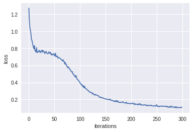
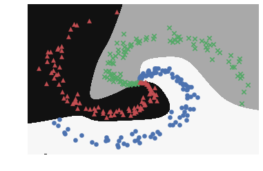
学習曲線と決定境界がほぼほぼ再現できたので、動作に関しても問題なしかと。
train_custome_loop.ipynb
# kerasはデフォルトで入っていないので、install
!pip install keras

%matplotlib inline
import numpy as np
import matplotlib.pyplot as plt
from keras.models import Sequential
from keras.layers import Dense
from keras.optimizers import SGD

# spiral.pyをcolab上でimportするのが手間なので、べた書き
def spiral_load_data(seed=1984):
 np.random.seed(seed)
 N = 100 # クラスごとのサンプル数
 DIM = 2 # データの要素数
 CLS_NUM = 3 # クラス数

 x = np.zeros((N*CLS_NUM, DIM))
 t = np.zeros((N*CLS_NUM, CLS_NUM), dtype=np.int)

 for j in range(CLS_NUM):
 for i in range(N):#N*j, N*(j+1)):
 rate = i / N
 radius = 1.0*rate
 theta = j*4.0 + 4.0*rate + np.random.randn()*0.2

 ix = N*j + i
 x[ix] = np.array([radius*np.sin(theta),
 radius*np.cos(theta)]).flatten()
 t[ix, j] = 1

 return x, t

# ハイパーパラメータの設定
max_epoch = 300
batch_size = 30
hidden_size = 10
learning_rate = 1.0

x, y = spiral_load_data()

## ↓ 大きな変更点 ↓
# モデルの宣言
model = Sequential()
model.add(Dense(hidden_size, activation='sigmoid', input_dim=x.shape[1]))
model.add(Dense(y.shape[1], activation='softmax'))
model.compile(optimizer=SGD(lr=learning_rate), loss='categorical_crossentropy')

hist = model.fit(x, y, epochs=max_epoch, batch_size=batch_size)
## ↑ 大きな変更点 ↑

# 学習結果のプロット
loss_list = hist.history['loss']
plt.plot(np.arange(len(loss_list)), loss_list, label='train')
plt.xlabel('iterations')
plt.ylabel('loss')
plt.show()

# 境界領域のプロット
h = 0.001
x_min, x_max = x[:, 0].min() - .1, x[:, 0].max() + .1
y_min, y_max = x[:, 1].min() - .1, x[:, 1].max() + .1
xx, yy = np.meshgrid(np.arange(x_min, x_max, h), np.arange(y_min, y_max, h))
X = np.c_[xx.ravel(), yy.ravel()]
score = model.predict(X)
predict_cls = np.argmax(score, axis=1)
Z = predict_cls.reshape(xx.shape)
plt.contourf(xx, yy, Z)
plt.axis('off')

# データ点のプロット
N = 100
CLS_NUM = 3
markers = ['o', 'x', '^']
for i in range(CLS_NUM):
 plt.scatter(x[i*N:(i+1)*N, 0], x[i*N:(i+1)*N, 1], s=40, marker=markers[i])
plt.show()
Register as a new user and use Qiita more conveniently
- You get articles that match your needs
- You can efficiently read back useful information
- You can use dark theme