
Bayesian method (1)
The prior distribution
It is easy to find a huge amount of good articles on the introduction of Bayesian statistics. However, most of them introduce only what Bayesian statistics is and how does Bayesian inference work and not many mathematical details are involved. In addition, it is a fun and challenging area to explore.
Therefore, I am planning to make a series of articles to share more about the theory of Bayesian statistics, which will include the selection of the prior, the loss function in the Bayesian inference and the relation between Bayesian statistics and some frequentists approaches. In this post, the prior distribution used in Bayesian statistics will be introduced. Why do we need to learn this? Because picking a prior distribution is one first steps we need to use Bayesian inference. And knowing more about them helps with choosing.
The basics
Here we start with a brief overview of how Bayesian statistics works and some notations we will use later are also introduced here. In Bayesian statistics, we assume a prior probability distribution and then update the prior using the data we have. This updating gives us the posterior probability distribution. We denote the posterior probability as π(θ|x) (π might seem to be very annoying since it’s also a very common constant in math, but in this context, π reminds us that the distribution is related to the parameter of the population distribution), and it is calculated as
where Θ is the space (here, by "space", we mean a "sample space") of all the possible parameters values and π(x|θ) is the likelihood – the conditional probability that given the true parameter value being θ, output x is observed. Since θ∈Θ is the parameter related to the _prior distributio_n, instead of the distribution of the population, we can θ the hyperparameter. And like always, we use the bold font (x) to denote a vector. The denominator is also known as the evidence, which is a normalizing factor (a constant) to make the posterior probability π(θ|x) be a probability distribution (sum up to one). This is very easy to verify
And the normalizing factor can be ignored in inference, we can see this in some pieces of literature, such as [1], since leaving out the constant doesn’t change the shape of the curve.
Then the prior probability can be written in the form
Once we have the posterior distribution, which is the distribution of the parameter (keep this in mind), we can calculate the predictive distribution. It is a conditional probability, which is the probability distribution of observing y, given data x. It is calculated as
where the red part is the probability density function of the new observation, given the parameter θ. Equation 1.3 might seem a bit messy at first, but after a close look, we can see that it’s in fact calculated using the law of total probability (which is as simple as a weighted average) – it is the integration of the product of the probability distribution of Y given the parameter value θ and __ the probability of the parameter taking value θ given data x.
Choosing the prior
The prior is sometimes described as the "belief" about the data. [2] This means that we choose the prior according to our knowledge of the data. Of course, it’s not completely a subjective matter as the word "belief" might suggest.
Properties of the prior
Note that the distribution of the parameter can be unbounded, which means that the probability densities of it are nonnegative, but their sum or integral is infinite. We call this kind of distribution of the parameter improper prior distribution.
According to Wikipedia, an informative prior expresses specific, definite information about a variable. Usually, it is avoided at all costs, but if prior information is available, the informative priors are an appropriate way of introducing the information into the model. [7]
When we don’t know much about our data and the distribution of the parameter, it makes sense to choose a so-called "vague prior", which reflects minimal knowledge. Therefore, we need a prior distribution with no population base, which makes it difficult to construct, and plays a minimal role in the posterior distribution. Such prior density is called noninformative prior, or diffuse prior. And some people rather think that the prior distribution always contains some information. Sometimes improper priors are used to represent such vague prior. Later we will see examples of this.
A related term is weakly informative prior, which contains partial information, which means it’s enough to give the posterior distribution reasonable bounds, but doesn’t fully capture one’s scientific knowledge about the parameter. [3]
A very interesting property of the prior is conjugacy, which means that the posterior distribution has the same parametric form as the prior distribution. We can see that this kind of prior is strongly related to the posterior, thus we say that it contains strong prior knowledge. [5] The benefit of conjugate priors is obvious – the posterior distribution will be a known distribution.
Examples of some common priors
- Uniform prior
The most intuitive and easiest prior is a uniform prior distribution if the value of the parameter is bounded. This prior is noninformative (sometimes it’s also called "a low information prior" [2]), it assumes that all the parameters in the parameter space Θ are equally likely. For example, if we want to use Bernoulli distribution to model the data (as in the famous example – coin tossing), the parameter p is a probability, which falls in the interval [0, 1]. In this case, the prior probability becomes π(θ) = 1, for θ in [0, 1].
- Haldane prior
Minimal knowledge doesn’t necessarily have to mean that all the parameters are equally likely. A lot of other noninformative priors are also possible. Another example of the noninformative prior is Haldane prior, which is proposed by J. B. S. Haldane for the estimation of rare events. The Haldane prior is actually the beta distribution with parameter α=0, β=0. Therefore the Haldane prior is
where B(α, β) is the beta function. As a reminder, the Beta function looks like this:
which can be also written in terms of the gamma function
Note that Beta(0,0) is not defined, but we can consider what it approximates to at point (0,0), which is shown in the following graph
The posterior distribution π(θ|x) is proportional to θ⁻¹(1-θ)⁻¹ (recall that the Bayesian theorem can be written in the form Equation 1.2), which means
This prior gives the most weight to θ=1 and θ=0. This can be made clear using the example from [5]: consider the scenario that we are observing whether an unknown compound will dissolve in water. At first, we are completely ignorant of the result. Therefore, after observing that a small sample dissolves, we immediately assume that all the samples will do so; if it doesn’t, we assume that no sample can dissolve.
- Conjugate prior – beta distribution
A third example is the beta distribution, it is a conjugate prior of the binomial distribution. And note that, since the Bernoulli distribution is a special case of the binomial distribution (the same as B(1, 1)), Beta distribution is also a conjugate prior of the Bernoulli distribution. It is a typical example of conjugate prior (it has appeared on Wikipedia, [3] and ).
Here we will show why the beta distribution is conjugate to the binomial distribution. Firstly recall that the probability mass function of the binomial distribution is
where n is the total number of trials, k is the number of successes and p is the probability of success. Therefore, the likelihood is
Referring to what we have seen in the section of basics, the likelihood is denoted as π(x|θ), where x is the observed value, so x = (k, n-k). This means
the parameters of the binomial distribution become the observed value and the "parameter" in this likelihood is the hyperparameter.
Then we choose beta distribution to be the prior. What we want to do is to show that the posterior distribution is the same type as the prior distribution.
The posterior distribution is derived as follows
we can see that the posterior distribution is again beta distribution.
4. Jeffreys Prior
The Jeffreys prior is a non-informative prior defined in terms of the square root of the determinant of the Fisher information matrix.
The Fisher information and Fisher information matrix were introduced here, but for convenience, we also mention it again here. Originally, the Fisher information is defined as the variance of the score
where the lower index θ means that the expected value is with regard to θ, and the matrix form is written as
but under some certain conditions (the density function f being second-order differentiable and regularity conditions, a good summary of which can be found here).
Equation 2.14 is the formula for the single variable case (when there are multiple parameters, we use the matrix form). Let’s try to calculate the Jeffreys prior of a Bernoulli trial, which is a single variable case. There are reasons why we use this distribution for demonstration, which we will see later. We know that the probability distribution of the Bernoulli distribution is
Now we need to calculate the Fisher information of the density function (Equation 2.15)
Since the parameter is just one-dimensional (single-variable), the Fisher information is just a number, which is also the determinant, and we have the prior distribution
Look at Equation 1.27 carefully and we will find out that the Jeffreys prior is similar to the Haldane prior. But unlike Haldane prior, Jeffreys prior is proper. The plot of Equation 1.27 looks as follows
It is also related to the Beta distribution since Equation 1.27 equals Beta(1/2, 1/2).
Summary
This post is mainly about the prior distribution in Bayesian inference. In the beginning, the basics of Bayesian inference are briefly introduced. Then we look at the types of the prior distributions and then some common prior distributions are selected.
References:
[1] Lee, T. S., & Mumford, D. (2003). Hierarchical Bayesian inference in the visual cortex. JOSA A, 20(7), 1434–1448.
[2] Surya, Tokdar, Choosing a prior distribution, accessed 4 December 2021.
[3] Gelman, A., Carlin, J. B., Stern, H. S., & Rubin, D. B. (1995). Bayesian data analysis. Chapman and Hall/CRC.
[4] Etz, A., & Wagenmakers, E. J. (2017). JBS Haldane’s contribution to the Bayes factor hypothesis test. Statistical Science, 313–329.
[5] Jaynes, E. T. (1968). Prior probabilities. IEEE Transactions on systems science and cybernetics, 4(3), 227–241.
[6] Stanford, J. L., & Vardeman, S. B. (1994). Statistical methods for physical science (Vol. 28). Academic Press.
[7] Golchi, S. (2016, October). Informative priors and Bayesian computation. In 2016 IEEE international conference on data science and advanced analytics (DSAA) (pp. 782–789). IEEE.
[8] Nicenboim, B., Schad, D. J., & Vasishth, S. (2021). An introduction to bayesian data analysis for cognitive science.
[9] Jeremy Orloff and Jonathan Bloom, _Conjugate priors: Beta and normal_, accessed 11 December 2021.
[10] _The prior distribution_, accessed 1 January 2022.
Further reading:
For more about probability theory:
For more about the comparison between Bayesian and frequentist approaches:
Supplement:
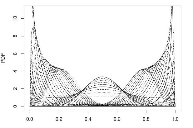
code used to generate Figure 0.1
x.v <- seq(0, 1, by=0.01)
n <- length(x.v)
m <- matrix(nrow=n, ncol=1)
for (i in seq(0.1, 5, 0.3)) {
y.v <- dbeta(x.v, shape1=i, shape2=15)
m <- cbind(y.v, m)
}
for (j in seq(0.1, 5, 0.3)) {
y.v <- dbeta(x.v, shape1=15, shape2=j)
m <- cbind(y.v, m)
}
for (i in seq(0.1, 10, 1)) {
y.v <- dbeta(x.v, shape1=i, shape2=i)
m <- cbind(y.v, m)
}
n.c <- ncol(m)
n.c
# remove last column with Nas
m <- m[,-n.c]
par(mar = c(3, 4, 1, 2))
matplot(x=x.v, y=m, type="l", col="black", ylim=c(0,11), xlab="", ylab="PDF")Share This Article
Towards Data Science is a community publication. Submit your insights to reach our global audience and earn through the TDS Author Payment Program.
Write for TDS