Entertainment

Data for Change

👁 Photo by Jon Tyson on Unsplash

Table of Content

· Data Collection ∘ Using an API to fetch data ∘ Data Wrangling ∘ Dataset Update · Data Analysis & Visualization ∘ Understanding the Bechdel data ∘ Comparing on-screen & off-screen metrics · Conclusions · References & Related Readings

---

As a big fan of movies and TV shows, I was intrigued when I first learned about the Bechdel Test in class. It measures the representation of women in fiction by checking 3 criteria:

• The movie has to have at least 2 [named] female characters
• who talk to each other
• about something other than a man.

This test was invented by Alison Bechdel in 1985, but it is still relevant in the present day. I expected it to be a simple test that all movies should pass, but is that the reality?

Before knowing what the Bechdel Test is, I would think about metrics such as if the director is a woman or the percentage of female cast members when talking about female representation in movies. These are off-screen representation metrics, while the Bechdel Test gives us a guideline for on-screen female representation, something that is rather difficult to quantify.

Therefore, to further investigate this topic and bridge the gap between on-screen and off-screen metrics, I obtained the Bechdel Test data on 9,300+ movies from this amazing website called Bechdel Test Movie List to answer the following questions:

• How do Bechdel Test scores change over time? Are movies doing better at passing the Bechdel Test 🤞?
• How does the Bechdel Test compare with other benchmarks of off-screen representation?

Check Kaggle for the dataset. Code in this post can be found in this GitHub repo.

Data Collection

All credits of the Bechdel Test data go to Bechdel Test Movie List, which provides a handy API for anyone to retrieve the raw data. The data comes with a CC BY-NC 3.0 license. We’re grateful to bechdeltest.com for the permission to use the data in this post.

Using an API to fetch data

The API documentation gives us 4 methods to call the data:

1. getMovieByImdbId (returns one movie with 9 columns)
2. getMoviesByTitle (returns multiple movies with matching title, 9 columns)
3. getAllMovieIds (returns all movies in database, 2 columns)
4. getAllMovies (returns all movies in database, 5 columns)

We can see right away that simply using one method will not give us all the information in the database. A dataframe of all information should probably contain all movies with 9 columns, so what are the missing 3 features from method #4 getAllMovies? Well, let’s check what getAllMovies really get us.

# import library 
import pandas as pd 
# get dataframe 
df = pd.read_json('http://bechdeltest.com/api/v1/getAllMovies') 
# check the last 5 rows of the dataframe 
df.tail() 
# you can check the first 5 rows by running df.head()

# save dataframe to a csv file
df.to_csv('Bechdel.csv')

👁 Image by Author

The movies are added chronologically, so the more recent ones are at the bottom. And we can see that Cruella does not have an imdbid, which is a problem we need to fix later.

The useful information method #4 getAllMovies gives us are movie title, IMDb id, unique website id (id), Bechdel Test score (rating), and year of release. The Bechdel test score, or rating, is calculated by checking the 3 criteria. Since each criterion is built upon the previous one, ie. a movie cannot fulfill criterion #2 if criterion #1 is not met, a score of 0 means a movie does not have 2 female characters. 1 means a movie has 2 female characters but they do not talk to each other. 2 means a movie has 2 women talking but they talk about men. 3 means completely passing the Bechdel Test. So, congrats to Cruella, West Side Story, Every Time a Bell Rings, and Single All The Way!

Now let’s see what method #1 getMovieByImdbId gives us.

# Using Single All The Way as an example (imdbid=14315756) pd.read_json('http://bechdeltest.com/api/v1/getMovieByImdbId?imdbid=14315756', typ='series')

👁 Image by Author

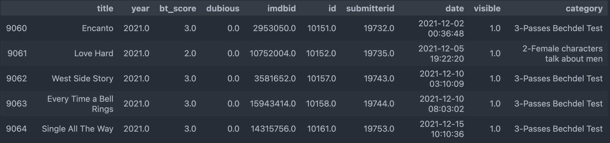
It does not have an index but has 4 additional columns: visible, date of the movie being added to the list, dubious, and submitter id. Visible is always 1 for every movie because only the visible movies are returned by the API call. What is interesting is the dubious column. It indicates "whether the submitter considered the rating dubious". In other words, we cannot trust the ratings of dubious movies, as they are susceptible to modification.

And this complicates things… dubious is now too important a column to ignore. We may discard the dubious movies, or we may treat dubious as another category. Either way, the df we have now needs a new column – dubious. And that took me an extra 7 hours.

Data Wrangling

Now that we have the IMDb id of each 9,300+ movies, we can use it to get the full information on each movie, which means we need to call the API thousands of times. The website states that:

Please keep in mind I’m running this site on a shared hosting plan, so if you send lots of queries in a short time, you might get me in trouble. Please be nice and definitely don’t use this data on anything with a lot of traffic.

I don’t want to cause any trouble, so I called the API every few seconds (hence it took me 7 hours). I did experience some timeout errors and unstable internet (that’s my bad), so maybe a few seconds was still too frequent. But thankfully, the website did not crash. For this reason, I suggest checking out this Kaggle database if you want to use the dataset and avoid calling the API again and causing more unnecessary traffic.

But the code to get the extra 4 columns is here:

However, we are not done yet. If we check the Bechdel_detailed.csv file, we will see 3 new columns and some NANs.

bechdel_detailed_df = pd.read_csv('Bechdel_detailed.csv', index_col=0) 
bechdel_detailed_df.info()

👁 Image by Author

A lot of dubious are NAN because the website returns null in their API, but there are 9373–9369=4 movies that seems strange. Let’s take a look at them.

bechdel_detailed_df[bechdel_detailed_df['title'].isna()]

👁 Image by Author

No surprise here because index 9369 is Cruella, which does not have an imdbid. We expected it to cause problem and now it’s time to fix it. We can go to IMDb and manually get the imdbid. Now, just a bit more data cleaning and we are done.

The current Bechdel_detailed.csv file should look like this. It contains 9,373 movies from year 1874 to 2021.

👁 Image by Author

Dataset Update

The website is updated quickly and the analysis here is based on the data from Dec. 23, 2021. Please check Kaggle for the latest dataset (I intend to maintain it quarterly).

Data Analysis & Visualization

As always, for any dataset, we start from exploratory data analysis (EDA) and visualize the data to get a sense of what we are dealing with.

Understanding the Bechdel data

Continuing where we left off, let’s first import more libraries and check the basic information of bechdel_detailed_df again.

# import libraries 
import numpy as np 
import matplotlib.pyplot as plt 
%matplotlib inline 
from plotnine import * 
from mizani.formatters import percent_format 

# rename column because the name rating a little confusing
bechdel_detailed_df.rename(columns={'rating': 'bt_score'}, inplace=True)

# check null 
bechdel_detailed_df.info()

👁 Image by Author

There are some dubious = NaN in the dataset, but not too many, so we can go ahead and drop them.

# drop NAN 
bechdel_detailed_df = bechdel_detailed_df.dropna().reset_index(drop=True)

len(bechdel_detailed_df) # returns 9074

Now, we have 9,074 movies in total. We also need to check duplicates and drop the 9 duplicated movies.

bechdel_detailed_df.duplicated().sum() # returns 9
bechdel_detailed_df.drop_duplicates(inplace=True) 
# reset index
bechdel_detailed_df = bechdel_detailed_df.reset_index(drop=True)
# left with 9,065 movies

Okay, we can start to visualize. Since I have been learning R in the past few months (my native language is Python), I have started to love the ggplot2 style, so I chose to use a mixture of matplotlib and plotnine for visualization.

First, I am curious about the score distribution and percentages in the dataset.

👁 Image by Author

More than half of the movies pass the Bechdel Test, which is quite disappointing considering the Bechdel Test does not seem too difficult to pass. However, fivethirtyeight says that the ~56% passing rate is already higher than expected [1]. They also point out a "feminist-leaning" problem, which means that people subconsciously pick the movies that are more likely to pass the Bechdel Test, because they know in advance that they are going to submit a score to the Bechdel website [1]. Also, it is not difficult to see that most of the movies in the database are popular Hollywood movies, which puts a geolocation restriction to our analysis as well.

It is important to acknowledge the biases in datasets and EDA helps us do that.

Let’s continue by dealing with dubious movies. Please recall that dubious movie scores are susceptible to changes and we have dropped the rows with dubious = nan, so now we are interested in the movies marked dubious = 1.

dubious_count = bechdel_detailed_df['dubious'].value_counts()

print('Percentage of dubious movie scores:', str('{:.2f}'.format(dubious_count[1.0] / (dubious_count[1.0] + dubious_count[0.0]) * 100))+'%')

Percentage of dubious movie scores: 8.92%

~9% is not too bad, but I don’t think we should drop the dubious movies right now. Instead, I intend to treat it as a new category at the same level as bt_score = 0, 1, 2 and 3. Let’s create another column called "category" and mark the 5 possibilities:

• Dubious
• 0-Fewer than two female characters
• 1-Female characters do not talk
• 2-Female characters talk about men

• 3-Passes Bechdel Test

  👁 Image by Author
  

Alright, let’s go on to analyze the trend over the years. We can calculate the mean score of each year and visualize in a scatter plot.

👁 Image by Author

I added a smooth curve so that it is easier to see the trend. Movies in the early years are performing extremely poorly, but the mean score is improving over time. Recent years have seen an all-time high.

Is it because the proportion of movies passing the test is increasing? Let’s find out.

I chose to use an animated pie chart for visualization because it shows the time flow nicely (fitting ~150 years in a bar chart looks terrible). Plus, it’s good to practice something new. And this time, I color-coded the 5 categories.

👁 GIF by Author (Animated graphs can show changes over time very nicely)

We can see that the early years are all orange, meaning that 0 movies pass the test. But over the years, more green color is popping up, meaning that more movies pass the test. However, the green proportion is unstable, because the interval of 1 year is too small. So, let’s use an interval of 10 years instead. And this time, we can finally fit everything in a bar chart.

👁 Image by Author (It's a percentage stacked bar chart that shows proportion, not a common bar chart that shows frequency, or counts.)

Dubious movies are in the middle so that the human eyes can better compare the green and the orange proportions. We can see that as the green proportion is getting bigger, the orange proportion is getting lighter. That is, many movies still fail the test, but more are getting 1’s and 2’s instead of 0’s, which shows progress. Yay!

Now, I want to take some time to emphasize that the terms "more" or "fewer" here are all in terms of proportion, or percentage, or ratio. They do not refer to the pure number, or volume, or quantity of the movies. Comparing numbers is meaningless. Why? Because of the population effect, or the size effect.

For example, there might be more movies (in terms of number) passing the Bechdel test in the year 2122 than 2022 simply because the year 2122 has 10 times more movies released than 2022. The proportion may drop, even if the number rises, so numbers alone do not tell us much useful information. Another example I heard recently is that a friend of mine is doing NLP and he found that the negative comments in sentiment analysis tend to be shorter, but the reason could be there are more short comments (in terms of number) on the internet in general, so his conclusion might not be meaningful. This pitfall has the term "population" in it because it is commonly associated with population. China has more births than Japan simply because China has a larger population. This is not interesting. What is interesting is the birth rate, not the birth number. Similarly, we talk about GDP per capita, not GDP as a whole. It is surprising how often we misinterpret the population effect as something meaningful.

Okay, let’s get back to the analysis. Now that we have a pretty good understanding of the Bechdel data and the general trend over time, let’s compare it with off-screen metrics.

Comparing on-screen & off-screen metrics

By off-screen metrics of female representation in movies, I mean the female ratios in cast and crew members. To get the ratios, we can use this popular Kaggle dataset. The credits.csv file marks the gender information.

👁 Image by Author

To join the Bechdel data with the gender data, we need the links.csv file.

# import more libraries
import ast 
from collections import defaultdict
import seaborn as sns

# load the 2 new datasets 
links_df = pd.read_csv('./TheMoviesData/links.csv', index_col=0) 
credits_df = pd.read_csv('./TheMoviesData/credits.csv')
# there are 37 duplicates in credits_df, but let's drop them later

# merge 
bechdel_df = pd.merge(bechdel_detailed_df, links_df, left_on='imdbid', right_on='imdbId', how='inner').drop(columns=['imdbId']) 

bechdel_df = pd.merge(bechdel_df, credits_df, left_on='tmdbId', right_on='id', how='inner').drop(columns=['imdbid', 'submitterid', 'date', 'visible', 'tmdbId', 'id_x', 'id_y']) 

bechdel_df

👁 Image by Author

There are some empty values in cast and crew. Let’s calculate the percentage of empty values and see what we should do.

count1, count2 = 0, 0 
for index, row in bechdel_df.iterrows():
 cast_list = ast.literal_eval(row['cast'])
 crew_list = ast.literal_eval(row['crew'])
 if len(cast_list) == 0:
 count1 += 1
 if len(crew_list) == 0:
 count2 += 1 

print('Empty cast percentage:', str('{:.2f}'.format(count1/len(bechdel_df) * 100))+'%') 

print('Empty crew percentage:', str('{:.2f}'.format(count2/len(bechdel_df) * 100))+'%')

Empty cast percentage: 0.41% Empty crew percentage: 0.11%

This is a very small percentage, so we can go ahead and drop them. Also, we need to drop duplicates.

bechdel_df = bechdel_df[(bechdel_df['cast'] != '[]') & (bechdel_df['crew'] != '[]')].reset_index(drop=True) 

# check & drop duplicates
print(bechdel_df.duplicated().sum()) # returns 9 bechdel_df.drop_duplicates(inplace=True)
bechdel_df = bechdel_df.reset_index(drop=True)

However, there is another problem of unknown genders in the Kaggle dataset. The original data source of the Kaggle dataset did not keep a detailed record on the gender information. In fact, there are a lot of unknowns.

Percentage of unknowns in Cast: 36.29% Percentage of unknowns in Crew: 59.01% Percentage of unknowns in Directing: 39.44% Percentage of unknowns in Writing: 38.91%

Since there are way too many unknowns, we can fill in the blanks by predicting gender from the first name. The gender-guesser package is a good choice [2]. This package treats gender as binary (could be a limitation) and tells us if a first name is male/female, or mostly male/female, or unknown/androgynous. For example, my name Chinese name Yuhan can belong to any gender and the package would tell you my gender is unknown, but you can tell from my English name Alison that I’m female.

Percentage of unknowns in Cast: 4.78% Percentage of unknowns in Crew: 4.99% Percentage of unknowns in Directing: 4.21% Percentage of unknowns in Writing: 4.99%

The percentages of unknown have dropped significantly, which is great! Now, it’s time to decide which metrics we want. The female ratios that I think are of importance are:

• Cast female ratio
• Crew female ratio
• Directing female ratio (there are director, assistant director, etc)
• Writer female ratio

So, we can add a new column by running:

bechdel_df['cast_female_ratio'] = gender_df['cast_female_num'] / gender_df['cast_total_num'] 

bechdel_df['crew_female_ratio'] = gender_df['crew_female_num'] / gender_df['crew_total_num'] 

bechdel_df['directing_female_ratio'] = gender_df['Directing_female'] / gender_df['Directing_total'] 

bechdel_df['writing_female_ratio'] = gender_df['Writing_female'] / gender_df['Writing_total'] 

bechdel_df.head()

👁 Image by Author

There are some NaN in the writing_female_ratio column because 0/0 is NaN. If the total number of writers is 0 (the denominator), then the records of these movies are probably incomplete and not useful to us. Let’s drop the null. Also, this time, we cannot consider the dubious anymore when comparing metrics, because dubious scores are not reliable.

bechdel_df_no_nan = bechdel_df.dropna().reset_index(drop=True) 
bechdel_df_no_nan_no_dubious = bechdel_df_no_nan[bechdel_df_no_nan['dubious']==0].reset_index(drop=True)

Now we can check the mean Bechdel score for each metric.

bechdel_df_no_nan_no_dubious.groupby('bt_score').mean()

👁 Image by Author

By eyeballing the means, it seems that a higher female ratio is correlated with a higher bt_score. To visualize the means and their uncertainty intervals, we can use error bars to compare the metrics with the Bechdel score. For cast female ratio vs Bechdel score, we have:

👁 Image by Author

The error bars do not overlap, which indicates that the means of the 4 groups where bt_score = 0, 1, 2 and 3 are statistically different. And the positive correlation is very obvious.

By changing the column name from cast_female_ratio to others, we can plot all 4 graphs.

👁 Image by Author

Groups failing the Bechdel test are not always different from each other, but they all have a lower female ratio compared to movies passing the test. The positive correlation between on-screen and off-screen metrics is quite salient. That is, the higher percentage of female members in the cast and crew, the more likely the movie is to pass the Bechdel Test, and vice versa. More female on set can indeed translate into a better female representation on screen.

And that’s the end of this fun analysis.

Conclusions

In this article, we have talked about:

• how to use an API to collect data
• how to make an animated pie chart
• what population effect/size effect is

We have answered these questions:

1. How do Bechdel Test scores change over time? Are movies doing better at passing the Bechdel Test?

Yes! The mean Bechdel score and the percentage of passing movie are rising. For the movies failing the Bechdel Test, more are closer to passing the test now.

2. How does the Bechdel Test compare with other benchmarks of off-screen representation?

There is a positive correlation between the Bechdel score and the female ratios in cast, crew, directing and writing. More females in the workplace can translate into a more feminist output.

The quantitative work here focuses more on data acquisition, data analysis, and visualization because this project is originally designed to explore the human-centeredness in Data Science. What’s important is learning to ask the right questions, identify biases and limitations, and be aware of why each decision was made on the dataset. I don’t think it makes much sense to, for example, predict the Bechdel score based on gender ratios and involve Machine Learning models in this project. Nor do I want to overcomplicate things by introducing statistical concepts like Tukey’s HSD for pairwise comparison if the visualization already says it all. But you are most welcome to do so if it suits your need.

My wonderful teammates JB, Min Jie and Fatima went through the comments on the Bechdel website and did the qualitative analysis that made the project whole. Please check here if you are interested!

Code in this post can be found in this GitHub repo. Check Kaggle for dataset.

References & Related Readings

Here are some articles that I found extremely helpful and inspirational when working on this project. They explore relationship between the Bechdel scores and other interesting aspects such as rating, budget, etc. Enjoy the fun read!

[1] https://fivethirtyeight.com/features/the-dollar-and-cents-case-against-hollywoods-exclusion-of-women/ [2] https://towardsdatascience.com/the-bechdel-test-analyzing-gender-disparity-in-hollywood-263cd4bcd9d

---

Special thanks to TDS editor Ben Huberman who is so incredibly helpful with getting the data license permission and guiding me through every step of publishing this article.

Thank you for reading! I hope this has been helpful to you. Please leave a comment if you have any feedback 🙂

Share This Article

• Share on Facebook
• Share on LinkedIn
• Share on X