Data Science

The "bite size" format of articles is meant to deliver concise, focused insights on a single, small-scope topic. After reading this article, you will understand (1) why homoscedastic errors are required for valid standard errors in linear regression and (2) how to calculate heteroscedastic robust errors and why they remove the need for the homoscedastic assumption.

Here are the contents of the article:

1. Quick overview of homo/heteroskedastic errors
2. Explanation of why the homoscedasticity assumption is needed in linear regression – going through the derivation in a friendly way 😃
3. How to modify the standard error formula to remove the homoscedastic assumption

Heteroscedastic vs Homoscedastic Errors

Heteroscedastic vs homoscedastic errors is a widely covered topic; if you have a good understanding of this, feel free to skip to the next section! I’ll give a very brief overview of it here – if you want to learn more, google is your friend!

People who have taken statistics 101 know that one of the key assumptions of linear regression is that the errors are homoscedastic. This means that the errors have a constant variance with relation to the target variable – or in clearer words, the model predicts consistently well for all levels of the target variable.

Here is what the two types of errors look like visually:

👁 Homoscedastic = constant variance in errors, Heteroskedastic = different variances of errors across values of x - image by author

Heteroscedasticity does not bias our coefficient estimates – this means that the distribution of our coefficient estimates is still centered on the actual mean of the true coefficient value. It does cause our standard errors to biased and often too small. Because of heteroscedasticity’s impact on our standard errors, we need to make adjustments to the standard error calculation if our data exhibits it.

Why is the homoscedasticity assumption needed?

In this section, we’ll see where the homoscedastic assumption comes into play in the derivation of the standard error formula. I’m not going to go through the full derivation of standard errors here (this is bite size remember!) – there are plenty of resources that cover that¹.

Let’s start out with the estimator for a coefficient:

👁 image by author

We make a bunch of transformations to the formula above to get a format that will be helpful for understanding where the homoscedastic assumption comes in. The transformed, equivalent formula is below:

👁 ϵ is the residual i.e., actual minus predicted - image by author

Now that we have our formula in a format that will prove friendly in a little bit, we are ready to take the variance of both sides to start our work calculating the standard error.

👁 image by author

Let’s clean the formula above— _β_1​ is constant and is independent from the rest of the formula. So we can pull it out of the variance function and get rid of it (remember the variance of a constant is 0).

We also treat the x values as constants. Using the "constant multiple rule," i.e., Var(aX)=_a²_Var(X), we can square the two summations and take them out of the variance.

These simplifying steps give us this formula:

👁 image by author

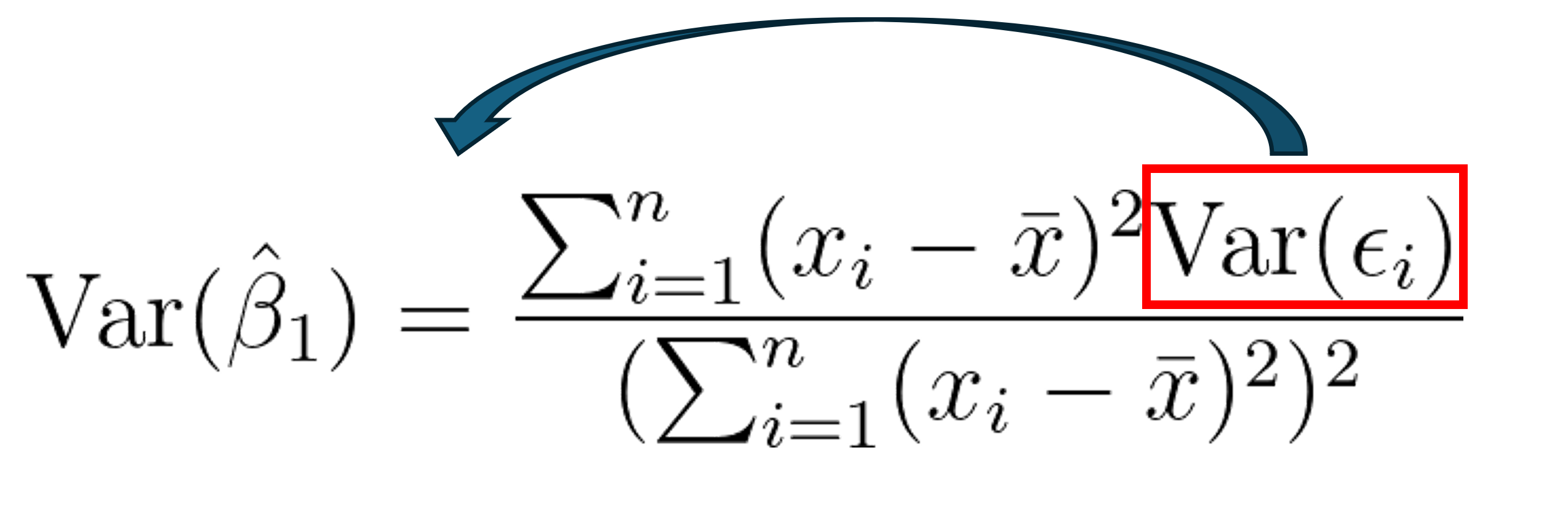
Okay, we have finally made it – this next part is where the homoscedastic assumption finally comes in!

Remember that multiplying by a constant inside of a summation is the same as multiplying the summation by a constant (distributive property of summation). If we assume that the variance of the error is constant (i.e., homoscedastic), we can use this rule to pull the variance of the errors out of the summation! This is it, this is where the homoscedastic assumption lies! Pretty exciting huh?!?

This is what the assumption looks like in the formula:

👁 image by author

We can’t observe var(ϵ) directly, but the variance of the residuals are an unbiased estimator of the variance of the error. So, we estimate the variance (note the hat above ‘var’ now) of the coefficient by replacing var(ϵ) with σ² in the numerator.

👁 image by author

This formula should be familiar. The square root of the function above is the coefficient’s standard error. Remember that to get here, we had to assume that the residuals are homoscedastic so we could pull the variance term out of the summation. Without it, we can’t get to the formula above!

Adjusting the formula to remove the heteroscedastic assumption

In the previous section, we found out exactly where the homoscedastic assumption comes into play. If our residuals are homoscedastic, we are all good to go. What if our residuals do not exhibit homoscedasticity? There are a few things we can do — in this article we will only talk about calculating heteroscedastic robust errors. This involves us going a different direction when we get to the point below in our calculations:

👁 image by author

Since var(ϵ) is not constant, we cannot take it out of the summation, which means we can’t simplify the fraction further. In the last step in the prior section, we used the variance of the residuals as an estimate for the variance of the error. We will do the same thing here, except instead of estimating a single error variance for the whole model, we will estimate a variance for every observation in our data. We do this by substituting the var(ϵ) with ϵ² for every x in the data.

Taking the square root of the formula below gives us the heteroskedastic robust standard deviation:

👁 image by author

So, if we have a way to modify the calculation that removes an assumption, why don’t we do this every time? One reason is that this doesn’t work well when you have a small data set. The intuition here is that, with homoscedastic errors, you are only estimating one var(ϵ) with an entire dataset. With the formula above, you are estimating a different var(ϵ) for each value of x. You need a lot more data to be able to estimate all of those variances well. If you have a large dataset and you see signs of heteroscedasticity in your errors, you can use robust standard errors to get a better standard error estimates.

Here is a summary graphic of what we covered in this article:

👁 Summary of derivations in article - image by author

1. https://youtu.be/XsyUzaZHs5o?si=zVZcnzEfHh9e_7-I

Share This Article

• Share on Facebook
• Share on LinkedIn
• Share on X