
Bokeh Interactive Plots: Part 2
How to guide to building a custom interactive Bokeh app
Overview
This is the second part of three part articles series covering Bokeh interactive visualizations. Since this article builds on the previous one, I recommended reading Part 1 first.
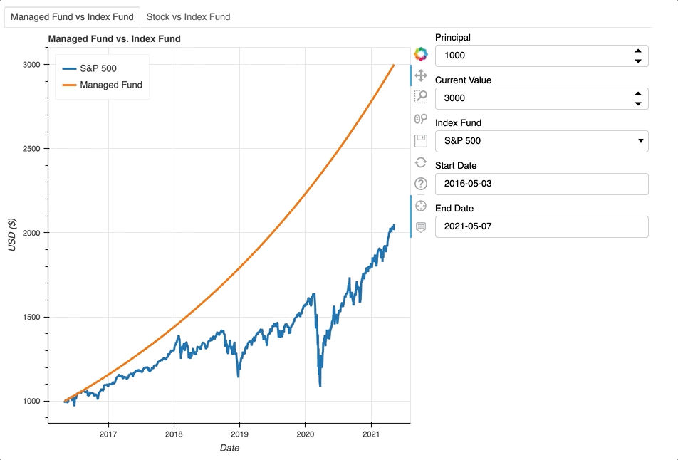
Part 1 built the Bokeh app framework to compare a managed fund and an index. Part 2 expands on that framework by adding the option to compare an index to any security available on the stock exchange such as EFTs, mutual funds, stocks, and index funds. The Part 2 capabilities are on a new tab in the app as shown below.
Part 2 aims to reuse as much of Part 1 as possible, but still requires some modifications to the functions. Since the Managed Fund vs. Index plot on Tab 1 still uses these functions, any additions must expand the functionality in a way that does not break the preexisting plot.
For the Stock vs. Index plot on Tab 2, both datasets depend on yf_fund because Yahoo Finance tracks both the index and the stock data.Thus, create_source and make_plot need to be retrofitted to work in cases where yf_fund generates both datasets. Before, create_source and make_plot took one input from yf_fund and the other from managed_fund.
Code
The Git Repository can be found here.
Widgets
Tab 2 uses a new type of widget, TextInput, which allows the user to input a security’s ticker symbol. Besides that, the other widgets on Tab 2 match the widgets on Tab 1. Since there are now two sets of widgets, dictionaries store the widgets rather than variables names. Instead of explicitly defining each widget, a loop defines the widgets. This method will prove helpful when editing update to work with both Tab 1 and Tab 2.
The dictionaries also store Dataframe and ColumnDataSource objects. Other functions will populate these dictionaries.
Functions
Part 2 introduces one new function, find_min_date. It takes tab_no and finds the minimum date for the tab’s plot. For Tab 1, the minimum date will depend on the when the index started. For Tab 2, the function checks when both the stock (fund_1) and the index (fund_2) began. The min_date for the Stock vs. Index plot on Tab 2 will be whichever date is more recent. The more recent date represents the beginning of when two assets’ timelines intersected. This is necessary because it’s not a fair comparison if one assets has more time to grow than the other. start_date_picker and end_date_picker widgets use min_date to set the minimum date a user can select.
Like in Part 1, yf_fund uses the Yahoo Finance module to pull in stock market data. Before, yf_fund only read in index data. Now, it also pulls in data given a ticker symbol. This could be a stock, mutual fund, or ETF. The only major addition to yf_fund is line 18 which factors in stock splits. Stock splits happen whenever a company decides to split an existing share of stock into multiple shares. For instance, when Amazon issued a 2–to-1 stock split in 1998, existing shareholders doubled their number of shares.
In Part 1, two different functions – managed_fund and yf_fund – generated the two inputs for create_source. However, to work with Part 2, create_source must also merge df_fund1 and df_fund2 even if yf_fund created both. If yf_fund creates both inputs, then the column names overlap. The rsuffix parameter in line 16 adds a suffix to the columns in df_fund2 to resolve the overlapping column names. lines 12and line 13 search through all the column names and identify which columns have data about the investments’ positions. Then, line 16 uses those columns to find the difference between the two investments
Line 6 and line 7 identify the names of the columns that hold the legend labels. Line 9 and line 10 rename the legend columns with more generic names. These generic names are necessary for make_plot. See make_plot for a more thorough explanation of why the columns need placeholder labels.
Similar to the changes in create_source, the edits in make_plot involve adding variables in order to identify the correct columns. make_plot is only called twice – once to make the Mutual Fund vs. Index plot on Tab 1 and then again to make the Stock vs. Index plot on Tab 2. As a result, sometimes the data will be in columns named Managed Position and Stock Position, and sometimes it will be in columns named Stock Position and Stock Position_2. position1 and position2 identify which columns contain the relevant data. label1 and label2 are the labels for the TOOLTIPS pop-up box.
In order to maintain proper formatting for TOOLTIPS, position1 and position2 must be added as f-strings. F-strings allow expressions to be embedded in a string as long as these embedded expressions are inside braces. TOOLTIPS also uses braces if a column name contains spaces. In order to properly work, each of the f-strings need three sets of braces. The f-string’s innermost pair indicates embedded information. The two outermost braces ensure the output string includes one set of braces. The output needs a set a braces because the column name contains a space. For example, if make_plot is called for the Tab 2 plot, the f-strings will output '{Stock Position}' and '{Stock Position_2}', and TOOLTIPS searchs for those column names.
create_source defined legend1 and legend2. They identify the columns in df_source that contains the ticker symbols. The legend uses those columns names as labels as shown on line 21 and line 23. As discussed in Part 1, Bokeh stores all updatable information in table format. Since the legend labels change whenever the user selects a new security, they must be in stored in columns.
The important thing to remember is make_plot is only called during initialization. It is not called each time the user changes an input and updates the data set. During updates, new data replaces the old data in source. Replacing the data in source changes the plot without calling make_plot.
Callback Function
update has a new argument, tab_no, because different tabs require different functions. For Tab 1, update calls managed_fund and yf_fund. For Tab 2, update only calls yf_fund. Then, create_source takes output data from managed_fund and/or yf_fund and merges the two Dataframes. After, the merged Dataframe is transformed into new_source, a ColumnDataSource object. Next, new_source replaces the data in source. To reiterate, updating the source is all that’s needed to change the displayed data.
Triggering Callbacks with Events
The callback function, update, needs to be linked to events. Changing widget values calls update. Bokeh callback functions only accept three arguments, attr, old, and new. However, now that the application has more than one tab, update needs know which tab to refresh. partial solves this dilemma. partial, which is part of the functools module, adds additional arguments to an existing function.
Case Study: S&P 500 vs. SPY
Since the Stock vs. Index plot has the capability to gather data about any tradable fund, the app can compare how an index fund measures up to the index it tracks. SPY is an ETF that tracks the S&P 500 index and one of the most popular ETF. Since its inception in 1993, SPY has averaged 10.5% annual return. As shown below, SPY mirrors the S&P 500 well, but not perfectly.
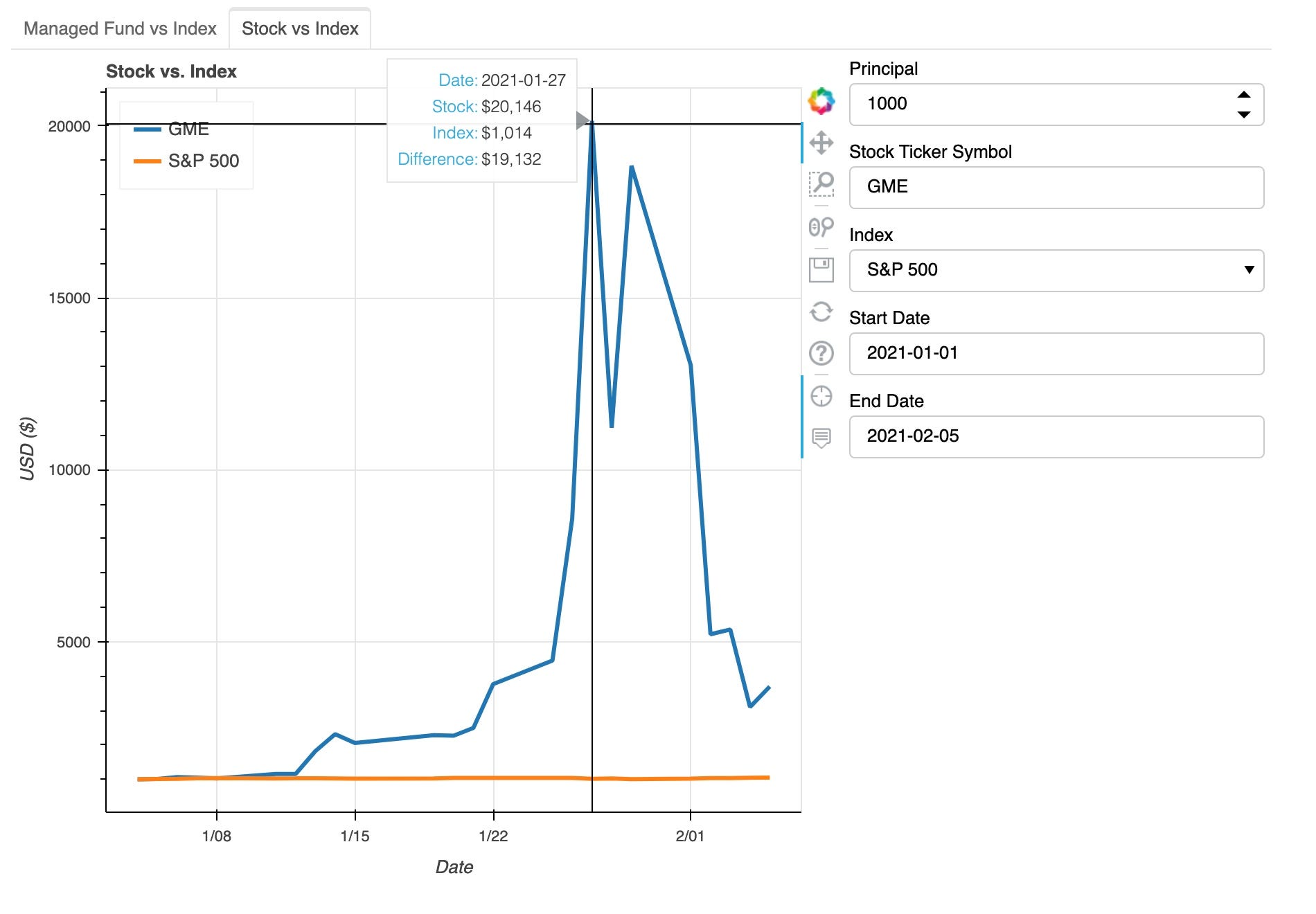
Case Study: S&P 500 vs. GME
Time in the market beats timing the market.
Last year, GameStop stock exploded. In short, many individual investors collectively decided to buy shares of GME which drove up demand and increased the stock price. Their crazy idea led to huge gains for the investors and huge losses for the many Wall Street hedge funds who shorted the stock.
GME rose so steeply that a $1000 investment would have yielded over $20,000 in less than 4 weeks. And then, the stock price took a sharp nosedive. Despite GME incredible growth in a span of a couple days, GME underscores the importance of not trying to time the market. Just ask anyone who bought high only to see the investment tank shortly after.
Next Steps
Part 3 adds a new tab with a Stock vs. Stock Plot and a text box which displays the appreciation of an investment, the difference between the two investments, and the cost basis.
https://medium.com/@katyhagerty19/bokeh-interactive-plots-part-3-683153f5f5ce
All feedback is welcome. I am always eager to learn new or better ways of doing things. Feel free to leave a comment or reach out to me at [email protected].
References
[1] Nickolas, Steven. SPY: SPDR S&P 500 ETF Trust (2021), Investopedia
Share This Article
Towards Data Science is a community publication. Submit your insights to reach our global audience and earn through the TDS Author Payment Program.
Write for TDS