Business

👁 Image from Unsplash by beasty

Join Medium with my referral link – Stefano Bosisio

When I was learning and get my hands dirty in machine learning, I always wondered how Google AutoML was able to pick up a suitable model for a given task, returning promising and encouraging metric results. Studying more and more, I was happy and excited when I found out the power of Neural Architecture Search (NAS), the key for creating new models, which is run underneath AutoML.

If on one side we have Deep Learning, which could be seen as a successful example of automating feature engineering – namely we do not have to spend hours for finding promising features as the architecture itself can handle this in the network – on the other side the next hopeful step for the ML future is to create automatically new powerful models. This step can be covered by NAS, which is getting a more and more exciting research field.

To understand NAS we must refer to Elsken, Metzen and Hutter review, which characterize NAS method into three steps:

• search space: This is a space where architecture principles live (e.g. CNN, LSTM, RNN and so on ). Prior knowledge of some architectures and tasks performance comes helpful to identify quickly new models, reducing the dimension of this space;
• search strategy: how can we explore the search space? The search strategy should give us rules on how to perform model research, with a compromise between finding a well-performing architecture quickly avoiding premature convergence;
• performance estimation strategy : we finally need a strategy to detect all the created architectures performances, satisfying the computational cost.

👁 Fig.1: dissecting NAS into three steps: 1) exploring the search space, where operations (e.g. pooling, convolution etc) live; 2) have a good detective strategy to pick the right bits and pieces for a specific tasks; 3) have an evaluator system for any created architecture. [Image by author.]

SEARCH SPACE

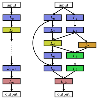
Naively we can think to populate our search space by creating NN architectures as a sequence of chain-structured neural networks. In this case, the i-th input of a layer _Li is the input for the layer L(i+1)._ Thus, we can think the phase space made of n maximum layers and any kind of operation for each layer, from convolution to pooling, along with any hyperparameter value associated to each operation. This is great, but the computational cost to search efficiently in such a space would be too demanding.

A second approach is the multi-branch network. Here we associate to each layer a function _g_i(L_i,…Lout) which allows the combination of the output from one layer to be the input for a random new layer. Furthermore, each branch is made up of cells: normal cells which preserve the dimensionality of the input and reduction cells which reduce the spatial dimension. By stacking together each cell we are creating the final architecture. Example for cells can be LSTM blocks or Convolutional architecture as well as RNNs.

👁 Fig.2: example of chain-structured neural network on the left and multi-branch network on the right. Image from the Elsken paper.

In coding terms, an initial attempt to implement a search space needs to answer these questions:

• what kind of architecture do we want to mimic? Can we start from architectures known by humans? Do we want to start with something new?
• how many layers do we want? Can we impose a limit?
• What computational power we have? How much does it cost?
• Which Python packages can I use? Keras? Tensorflow?

Just think this: although we might think of small neural networks, the number of parameters in the search space would be extremely high. To reduce the computational cost we could think of a list to be explored for the number of neurons in each hidden layers. From there, we can do the same for a set of activation functions. Finally, we could even think of inserting known architectures in the building functions:

SEARCH STRATEGY

Now that we have defined the building blocks of the search space we need a way to search for the right pieces. This is a fantastic field of research with a lot of vibrant and exciting ideas. Each new architecture can be built up based on Bayesian optimization or evolutionary methods, inspired by neuro-evolution (e.g. genetic algorithms). Another promising approach would be the reinforcement learning one, where the state is a partially trained architecture, the reward is the model’s performance and the action is a function-preserving mutations to the final model. Further recent examples are Monte Carlo Tree Search or hill climbing algorithm or continuous relaxation

In Python we could think of something similar for implementing the search strategy:

PERFORMANCE ESTIMATION

To further define a search strategy we need to find a suitable method to compute the performance metric for each created model. Naively we could think of running evaluation on all the generated models against training data, but this would require an immense computational cost, given the huge search space we are living on. However, we can find some solutions:

• lower fidelities: performance can be estimated on lower fidelities of the actual performance after full training. This can be training on a subset of data or lower resolution data or with fewer filters and cells per layer.
• extrapolation of learning curves: the performance can be extrapolated after just a few epochs of training from early generated learning curves
• predicting performances: another model can be used to predict the performance of the various architectures
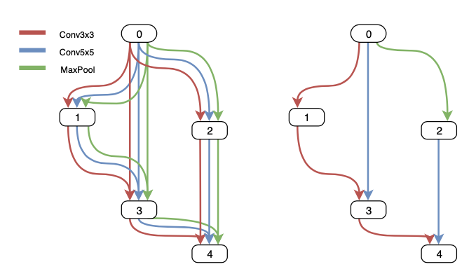
• one-shot architecture: this is a "graph" based procedure. For every created architecture, there is a one-shot model which contains different pieces of all the architectures (e.g. the CNN of one architecture 1, the LSTM of architecture 2 and so on). This model is then trained and its weights are shared across all the existing architectures and used to retrieve the performance

👁 Fig. 3: One-short architecture approach: the created architectures are shown on the left side. Rather than evaluating each single model, it is possible to evaluate a one-shot model with bits and pieces from all the architectures. From there, weights are shared among all the existing architectures. Image from the Elsken paper.

The one-shot architecture is widely used nowadays. It is obvious the efficiency we could get by training a super-network to then rank several candidates. However, often there is thorough post-processing to retrieve exact accuracy from each candidate. Weights need to be compensated, retrained and finetuned after the search. Sadly, these steps bring an additional computational cost, as well as complexity when it comes to the deployment phase. Indeed, each candidate has a different performance on different hardware. For example, even if two devices may have the same CPUs, as in the case in mobile phones, the hardware may prefer one network architecture, returning a different accuracy and performance. This engineering aspect brings us to the last step: how to deploy correctly a NAS model?

BigNAS: find suitable models for suitable hardware

One of the most ignored requirements in ML is being resource-aware. This means that we often need to minimize the resource usage, latency or FLOPs. Google Brain is tackling this issue with BigNAS, which can be seen as a 2-step process:

• Firstly, train a big single-stage model, whose weights are ready to be used at deployment time. Given the size of this model, it is possible to slice different child architectures, which comes in handy for instant inference and deployment on different hardware.
• Find the most accurate model, given hardware resource constraints (e.g. CPUs size, latency, budget)

BigNAS is a novel paradigm for NAS, which has proved to surpass state-of-the-art ImageNet classification models searches in a wide range of hardware architectures. To make BigNAS work we just need few simple steps:

• Sandwich Rule: this funny name was given by Yu and Huang, defining a strategy where for each iteration the smallest and the biggest model are trained. In BigNAS context, at each training step, a mini-batch of data is processed against the smallest child model and the biggest child model plus few other random child models. Then, all the gradients from the sampled child are aggregated and used to update the weights in the single-stage model
• Inplace Distillation: the idea here is to transfer the knowledge gained by the biggest model from real data to all the smaller children ones. In particular, the predicted labels from the biggest model are used as the training label for all the smaller child models.

Finally, the best model is chosen with a coarse-to-fine strategy. In this approach, initially, the rough skeleton of promising network candidates are searched and then sampled with fine-grained variations. In this setup, a limited input resolution set, depth set and kernel set are defined to benchmark models. Then, the best model is picked up and randomly mutated (e.g. network-wise resolution, stage-wise depth, kernel size) to improve more and more the final model.

This work helps to scale up further the NAS, which may bring us at some point to new and powerful architectures to solve more and more complicated tasks. However remember, there is always a price to pay, which is understanding what the model is doing and how the features come to play in the model’s decision process.

---

Please, feel free to send me an email for questions or comments at: [email protected]

Alternatively, you can contact me on Instagram: https://www.instagram.com/a_pic_of_science/

Share This Article

• Share on Facebook
• Share on LinkedIn
• Share on X