1. Overview

The run-time complexity of algorithms is often dependent on the nature of the input.

In this tutorial, we’ll see how the trivial implementation of the Quicksort algorithm has a poor performance for repeated elements.

Further, we’ll learn a few Quicksort variants to efficiently partition and sort inputs with a high density of duplicate keys.

2. Trivial Quicksort

Quicksort is an efficient sorting algorithm based on the divide and conquer paradigm. Functionally speaking, it operates in-place on the input array and rearranges the elements with simple comparison and swap operations.

2.1. Single-pivot Partitioning

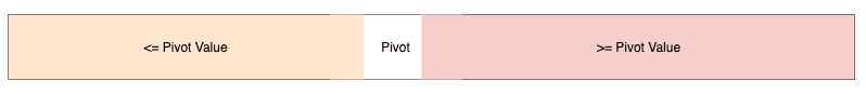
A trivial implementation of the Quicksort algorithm relies heavily on a single-pivot partitioning procedure. In other words, partitioning divides the array A=[a_p, a_p+1, a_p+2,…, a_r] into two parts A[p..q] and A[q+1..r] such that:

• All elements in the first partition, A[p..q] are lesser than or equal to the pivot value A[q]
• All elements in the second partition, A[q+1..r] are greater than or equal to the pivot value A[q]

After that, the two partitions are treated as independent input arrays and fed themselves to the Quicksort algorithm. Let’s see Lomuto’s Quicksort in action:

2.2. Performance with Repeated Elements

Let’s say we have an array A = [4, 4, 4, 4, 4, 4, 4] that has all equal elements.

On partitioning this array with the single-pivot partitioning scheme, we’ll get two partitions. The first partition will be empty, while the second partition will have N-1 elements. Further, each subsequent invocation of the partition procedure will reduce the input size by only one. Let’s see how it works:

Since the partition procedure has linear time complexity, the overall time complexity, in this case, is quadratic. This is the worst-case scenario for our input array.

3. Three-way Partitioning

To efficiently sort an array having a high number of repeated keys, we can choose to handle the equal keys more responsibly. The idea is to place them in the right position when we first encounter them. So, what we’re looking for is a three partition state of the array:

• The left-most partition contains elements which are strictly less than the partitioning key
• The middle partition contains all elements which are equal to the partitioning key
• The right-most partition contains all elements which are strictly greater than the partitioning key

We’ll now dive deeper into a couple of approaches that we can use to achieve three-way partitioning.

4. Dijkstra’s Approach

Dijkstra’s approach is an effective way of doing three-way partitioning. To understand this, let’s look into a classic programming problem.

4.1. Dutch National Flag Problem

Inspired by the tricolor flag of the Netherlands, Edsger Dijkstra proposed a programming problem called the Dutch National Flag Problem (DNF).

In a nutshell, it’s a rearrangement problem where we’re given balls of three colors placed randomly in a line, and we’re asked to group the same colored balls together. Moreover, the rearrangement must ensure that groups follow the correct order.

Interestingly, the DNF problem makes a striking analogy with the 3-way partitioning of an array with repeated elements.

We can categorize all the numbers of an array into three groups with respect to a given key:

• The Red group contains all elements that are strictly lesser than the key
• The White group contains all elements that are equal to the key
• The Blue group contains all elements that strictly greater than the key

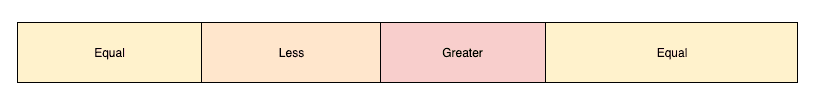
4.2. Algorithm

One of the approaches to solve the DNF problem is to pick the first element as the partitioning key and scan the array from left to right. As we check each element, we move it to its correct group, namely Lesser, Equal, and Greater.

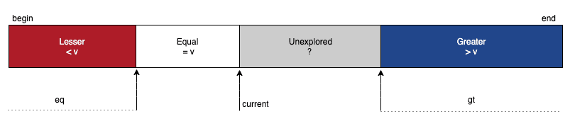
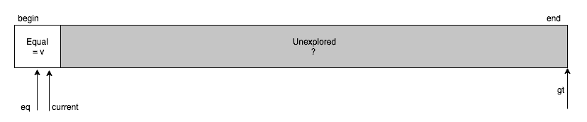
To keep track of our partitioning progress, we’d need the help of three pointers, namely lt, current, and gt. At any point in time, the elements to the left of lt will be strictly less than the partitioning key, and the elements to the right of gt will be strictly greater than the key.

Further, we’ll use the current pointer for scanning, which means that all elements lying between the current and gt pointers are yet to be explored:

To begin with, we can set lt and current pointers at the very beginning of the array and the gt pointer at the very end of it:

For each element read via the current pointer, we compare it with the partitioning key and take one of the three composite actions:

• If input[current] < key, then we exchange input[current] and input[lt] and increment both current and lt pointers
• If input[current] == key, then we increment current pointer
• If input[current] > key, then we exchange input[current] and input[gt] and decrement gt

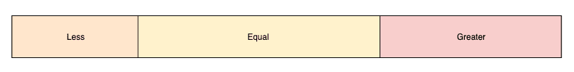
Eventually, we’ll stop when the current and gt pointers cross each other. With that, the size of the unexplored region reduces to zero, and we’ll be left with only three required partitions.

Finally, let’s see how this algorithm works on an input array having duplicate elements:

4.3. Implementation

First, let’s write a utility procedure named compare() to do a three-way comparison between two numbers:

public static int compare(int num1, int num2) {
 if (num1 > num2)
 return 1;
 else if (num1 < num2)
 return -1;
 else
 return 0;
}

Next, let’s add a method called swap() to exchange elements at two indices of the same array:

public static void swap(int[] array, int position1, int position2) {
 if (position1 != position2) {
 int temp = array[position1];
 array[position1] = array[position2];
 array[position2] = temp;
 }
}

To uniquely identify a partition in the array, we’ll need its left and right boundary-indices. So, let’s go ahead and create a Partition class:

public class Partition {
 private int left;
 private int right;
}

Now, we’re ready to write our three-way partition() procedure:

public static Partition partition(int[] input, int begin, int end) {
 int lt = begin, current = begin, gt = end;
 int partitioningValue = input[begin];

 while (current <= gt) {
 int compareCurrent = compare(input[current], partitioningValue);
 switch (compareCurrent) {
 case -1:
 swap(input, current++, lt++);
 break;
 case 0:
 current++;
 break;
 case 1:
 swap(input, current, gt--);
 break;
 }
 }
 return new Partition(lt, gt);
}

Finally, let’s write a quicksort() method that leverages our 3-way partitioning scheme to sort the left and right partitions recursively:

public static void quicksort(int[] input, int begin, int end) {
 if (end <= begin)
 return;

 Partition middlePartition = partition(input, begin, end);

 quicksort(input, begin, middlePartition.getLeft() - 1);
 quicksort(input, middlePartition.getRight() + 1, end);
}

5. Bentley-McIlroy’s Approach

Jon Bentley and Douglas McIlroy co-authored an optimized version of the Quicksort algorithm. Let’s understand and implement this variant in Java:

5.1. Partitioning Scheme

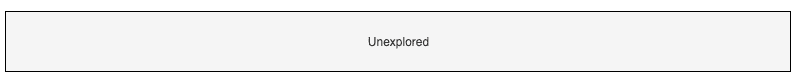
The crux of the algorithm is an iteration-based partitioning scheme. In the start, the entire array of numbers is an unexplored territory for us:

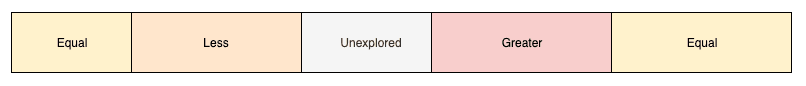
We then start exploring the elements of the array from the left and right direction. Whenever we enter or leave the loop of exploration, we can visualize the array as a composition of five regions:

• On the extreme two ends, lies the regions having elements that are equal to the partitioning value
• The unexplored region stays in the center and its size keeps on shrinking with each iteration
• On the left of the unexplored region lies all elements lesser than the partitioning value
• On the right side of the unexplored region are elements greater than the partitioning value

Eventually, our loop of exploration terminates when there are no elements to be explored anymore. At this stage, the size of the unexplored region is effectively zero, and we’re left with only four regions:

Next, we move all the elements from the two equal-regions in the center so that there is only one equal-region in the center surrounding by the less-region on the left and the greater-region on the right. To do so, first, we swap the elements in the left equal-region with the elements on the right end of the less-region. Similarly, the elements in the right equal-region are swapped with the elements on the left end of the greater-region.

Finally, we’ll be left with only three partitions, and we can further use the same approach to partition the less and the greater regions.

5.2. Implementation

In our recursive implementation of the three-way Quicksort, we’ll need to invoke our partition procedure for sub-arrays that’ll have a different set of lower and upper bounds. So, our partition() method must accept three inputs, namely the array along with its left and right bounds.

public static Partition partition(int input[], int begin, int end){
	// returns partition window
}

For simplicity, we can choose the partitioning value as the last element of the array. Also, let’s define two variables left=begin and right=end to explore the array inward.

Further, We’ll also need to keep track of the number of equal elements lying on the leftmost and rightmost. So, let’s initialize leftEqualKeysCount=0 and rightEqualKeysCount=0, and we’re now ready to explore and partition the array.

First, we start moving from both the directions and find an inversion where an element on the left is not less than partitioning value, and an element on the right is not greater than partitioning value. Then, unless the two pointers left and right have crossed each other, we swap the two elements.

In each iteration, we move elements equal to partitioningValue towards the two ends and increment the appropriate counter:

while (true) {
 while (input[left] < partitioningValue) left++; 
 
 while (input[right] > partitioningValue) {
 if (right == begin)
 break;
 right--;
 }

 if (left == right && input[left] == partitioningValue) {
 swap(input, begin + leftEqualKeysCount, left);
 leftEqualKeysCount++;
 left++;
 }

 if (left >= right) {
 break;
 }

 swap(input, left, right);

 if (input[left] == partitioningValue) {
 swap(input, begin + leftEqualKeysCount, left);
 leftEqualKeysCount++;
 }

 if (input[right] == partitioningValue) {
 swap(input, right, end - rightEqualKeysCount);
 rightEqualKeysCount++;
 }
 left++; right--;
}

In the next phase, we need to move all the equal elements from the two ends in the center. After we exit the loop, the left-pointer will be at an element whose value is not less than partitioningValue. Using this fact, we start moving equal elements from the two ends towards the center:

right = left - 1;
for (int k = begin; k < begin + leftEqualKeysCount; k++, right--) { 
 if (right >= begin + leftEqualKeysCount)
 swap(input, k, right);
}
for (int k = end; k > end - rightEqualKeysCount; k--, left++) {
 if (left <= end - rightEqualKeysCount)
 swap(input, left, k);
}

In the last phase, we can return the boundaries of the middle partition:

return new Partition(right + 1, left - 1);

Finally, let’s take a look at a demonstration of our implementation on a sample input

6. Algorithm Analysis

In general, the Quicksort algorithm has an average-case time complexity of O(n*log(n)) and worst-case time complexity of O(n²). With a high density of duplicate keys, we almost always get the worst-case performance with the trivial implementation of Quicksort.

However, when we use the three-way partitioning variant of Quicksort, such as DNF partitioning or Bentley’s partitioning, we’re able to prevent the negative effect of duplicate keys. Further, as the density of duplicate keys increase, the performance of our algorithm improves as well. As a result, we get the best-case performance when all keys are equal, and we get a single partition containing all equal keys in linear time.

Nevertheless, we must note that we’re essentially adding overhead when we switch to a three-way partitioning scheme from the trivial single-pivot partitioning.

For DNF based approach, the overhead doesn’t depend on the density of repeated keys. So, if we use DNF partitioning for an array with all unique keys, then we’ll get poor performance as compared to the trivial implementation where we’re optimally choosing the pivot.

But, Bentley-McIlroy’s approach does a smart thing as the overhead of moving the equal keys from the two extreme ends is dependent on their count. As a result, if we use this algorithm for an array with all unique keys, even then, we’ll get reasonably good performance.

In summary, the worst-case time complexity of both single-pivot partitioning and three-way partitioning algorithms is O(nlog(n)). However, the real benefit is visible in the best-case scenarios, where we see the time complexity going from O(nlog(n)) for single-pivot partitioning to O(n) for three-way partitioning.

7. Conclusion

In this tutorial, we learned about the performance issues with the trivial implementation of the Quicksort algorithm when the input has a large number of repeated elements.

With a motivation to fix this issue, we learned different three-way partitioning schemes and how we can implement them in Java.