Big O Notation

Big O notation is used to describe the time or space complexity of algorithms. Big-O is a way to express an upper bound of an algorithm’s time or space complexity.

• Describes the asymptotic behavior (order of growth of time or space in terms of input size) of a function, not its exact value.
• Can be used to compare the efficiency of different algorithms or data structures.
• It provides an upper limit on the time taken by an algorithm in terms of the size of the input. We mainly consider the worst case scenario of the algorithm to find its time complexity in terms of Big O

Big O Definition

Given two functions f(n) and g(n), we say that f(n) is O(g(n)) if there exist constants c > 0 and n₀ >= 0 such that f(n) <= c*g(n) for all n >= n₀.

In simpler terms, f(n) is O(g(n)) if f(n) grows no faster than c*g(n) for all n >= n₀ where c and n₀ are constants.

👁 big-o-image

A Quick Way to find Big O of an Expression

• Ignore the lower order terms and consider only highest order term.
• Ignore the constant associated with the highest order term.

Example 1: f(n) = 3n² + 2n + 1000Logn + 5000
After ignoring lower order terms, we get the highest order term as 3n²
After ignoring the constant 3, we get n²
Therefore the Big O value of this expression is O(n²)

Example 2 : f(n) = 3n³ + 2n² + 5n + 1
Dominant Term: 3n³
Order of Growth: Cubic (n³)
Big O Notation: O(n³)

Properties of Big O Notation

Below are some important Properties of Big O Notation:

1. Reflexivity

For any function f(n), f(n) = O(f(n)).

Example:

f(n) = n², then f(n) = O(n²).

2. Transitivity

If f(n) = O(g(n)) and g(n) = O(h(n)), then f(n) = O(h(n)).

Example:

If f(n) = n^2, g(n) = n^3, and h(n) = n^4, then f(n) = O(g(n)) and g(n) = O(h(n)).
Therefore, by transitivity, f(n) = O(h(n)).

3. Constant Factor

For any constant c > 0 and functions f(n) and g(n), if f(n) = O(g(n)), then cf(n) = O(g(n)).

Example:

f(n) = n, g(n) = n². Then f(n) = O(g(n)). Therefore, 2f(n) = O(g(n)).

4. Sum Rule

If f(n) = O(g(n)) and h(n) = O(k(n)), then f(n) + h(n) = O(max( g(n), k(n) ) When combining complexities, only the largest term dominates.

Example:

f(n) = n², h(n) = n³. Then , f(n) + h(n) = O(max(n² + n³) = O ( n³)

5. Product Rule

If f(n) = O(g(n)) and h(n) = O(k(n)), then f(n) * h(n) = O(g(n) * k(n)).

Example:

f(n) = n, g(n) = n², h(n) = n³, k(n) = n⁴. Then f(n) = O(g(n)) and h(n) = O(k(n)). Therefore, f(n) * h(n) = O(g(n) * k(n)) = O(n⁶).

6. Composition Rule

If f(n) = O(g(n)), then f(h(n)) = O(g(h(n))).

Example:

If , and , then by composition rule f(h(n))=O(g(h(n))). Therefore, .

Common Big-O Notations

Big-O notation is a way to measure the time and space complexity of an algorithm. It describes the upper bound of the complexity in the worst-case scenario. Let’s look into the different types of time complexities:

1. Linear Time Complexity: Big O(n) Complexity

Linear time complexity means that the running time of an algorithm grows linearly with the size of the input.

For example, consider an algorithm that traverses through an array to find a specific element:

2. Logarithmic Time Complexity: Big O(log n) Complexity

Logarithmic time complexity means that the running time of an algorithm is proportional to the logarithm of the input size.

For example, a binary search algorithm has a logarithmic time complexity:

3. Quadratic Time Complexity: Big O(n²) Complexity

Quadratic time complexity means that the running time of an algorithm is proportional to the square of the input size.

For example, a simple bubble sort algorithm has a quadratic time complexity:

4. Cubic Time Complexity: Big O(n³) Complexity

Cubic time complexity means that the running time of an algorithm is proportional to the cube of the input size.

For example, a naive matrix multiplication algorithm has a cubic time complexity:

5. Polynomial Time Complexity: Big O(n^k) Complexity

Polynomial time complexity refers to the time complexity of an algorithm that can be expressed as a polynomial function of the input size n. In Big O notation, an algorithm is said to have polynomial time complexity if its time complexity is O(n^k), where k is a constant and represents the degree of the polynomial.

Algorithms with polynomial time complexity are generally considered efficient, as the running time grows at a reasonable rate as the input size increases. Common examples of algorithms with polynomial time complexity include linear time complexity O(n), quadratic time complexity O(n²), and cubic time complexity O(n³).

6. Exponential Time Complexity: Big O(2ⁿ) Complexity

Exponential time complexity means that the running time of an algorithm doubles with each addition to the input data set.

For example, the problem of generating all subsets of a set is of exponential time complexity:

7. Factorial Time Complexity: Big O(n!) Complexity

Factorial time complexity means that the running time of an algorithm grows factorially with the size of the input. This is often seen in algorithms that generate all permutations of a set of data.

Here’s an example of a factorial time complexity algorithm, which generates all permutations of an array:

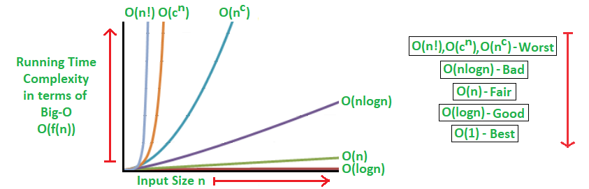
If we plot the most common Big O notation examples, we would have graph like this:

👁 asymtotic-analysis

Mathematical Examples of Runtime Analysis

Below table illustrates the runtime analysis of different orders of algorithms as the input size (n) increases.

Algorithmic Examples of Runtime Analysis

Below table categorizes algorithms based on their runtime complexity and provides examples for each type.