Longest Common Extension / LCE using Segment Tree

Prerequisites :

LCE(Set 1)

,

LCE(Set 2)

,

Suffix Array (n Log Log n)

,

Kasai's algorithm

and

Segment Tree

The Longest Common Extension (LCE) problem considers a string

s

and computes, for each pair (L , R), the longest sub string of

s

that starts at both L and R. In LCE, in each of the query we have to answer the length of the longest common prefix starting at indexes L and R.

Example:

String

: “abbababba”

Queries:

LCE(1, 2), LCE(1, 6) and LCE(0, 5) Find the length of the Longest Common Prefix starting at index given as,

(1, 2), (1, 6) and (0, 5)

. The string highlighted

“green”

are the longest common prefix starting at index- L and R of the respective queries. We have to find the length of the longest common prefix starting at index-

(1, 2), (1, 6) and (0, 5)

.

In this set we will discuss about the Segment Tree approach to solve the LCE problem. In

Set 2

, we saw that an LCE problem can be converted into a RMQ problem. To process the RMQ efficiently, we build a segment tree on the lcp array and then efficiently answer the LCE queries. To find low and high, we must have to compute the suffix array first and then from the suffix array we compute the inverse suffix array. We also need lcp array, hence we use

Kasai’s Algorithm to find lcp array from the suffix array

. Once the above things are done, we simply find the minimum value in lcp array from index low to high (as proved above) for each query. Without proving we will use the direct result (deduced after mathematical proofs)- LCE (L, R) = RMQ

_lcp

(invSuff[R], invSuff[L]-1) The subscript lcp means that we have to perform RMQ on the lcp array and hence we will build a segment tree on the lcp array.

Output:

LCE (1, 2) = 1
LCE (1, 6) = 3
LCE (0, 5) = 4

Time Complexity :

To construct the lcp and the suffix array it takes O(N.logN) time. To answer each query it takes O(log N). Hence the overall time complexity is O(N.logN + Q.logN)). Although we can construct the lcp array and the suffix array in O(N) time using other algorithms. where, Q = Number of LCE Queries. N = Length of the input string.

Auxiliary Space :

We use O(N) auxiliary space to store lcp, suffix and inverse suffix arrays and segment tree.

Comparison of Performances:

We have seen three algorithm to compute the length of the LCE.

Set 1 :

Naive Method [O(N.Q)]

Set 2 :

RMQ-Direct Minimum Method [O(N.logN + Q. (|invSuff[R] – invSuff[L]|))]

Set 3 :

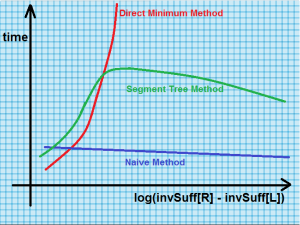
Segment Tree Method [O(N.logN + Q.logN))] invSuff[] = Inverse suffix array of the input string. From the asymptotic time complexity it seems that the Segment Tree method is most efficient and the other two are very inefficient. But when it comes to practical world this is not the case. If we plot a graph between time vs log((|invSuff[R] – invSuff[L]|) for typical files having random strings for various runs, then the result is as shown below.

👁 LCE

The above graph is taken from

this

reference. The tests were run on 25 files having random strings ranging from 0.7 MB to 2 GB. The exact sizes of string is not known but obviously a 2 GB file has a lot of characters in it. This is because 1 character = 1 byte. So, about 1000 characters equal 1 kilobyte. If a page has 2000 characters on it (a reasonable average for a double-spaced page), then it will take up 2K (2 kilobytes). That means it will take about 500 pages of text to equal one megabyte. Hence 2 gigabyte = 2000 megabyte = 2000*500 = 10,00,000 pages of text ! From the above graph it is clear that the Naive Method (discussed in Set 1) performs the best (better than Segment Tree Method). This is surprising as the asymptotic time complexity of Segment Tree Method is much lesser than that of the Naive Method. In fact, the naive method is generally 5-6 times faster than the Segment Tree Method on typical files having random strings. Also not to forget that the Naive Method is an in-place algorithm, thus making it the most desirable algorithm to compute LCE . The bottom-line is that the naive method is the most optimal choice for answering the LCE queries when it comes to average-case performance. Such kind of thinks rarely happens in Computer Science when a faster-looking algorithm gets beaten by a less efficient one in practical tests. What we learn is that the although asymptotic analysis is one of the most effective way to compare two algorithms on paper, but in practical uses sometimes things may happen the other way round.

References:

https://www.sciencedirect.com/science/article/pii/S1570866710000377

If you like GeeksforGeeks and would like to contribute, you can also write an article using

write.geeksforgeeks.org

or mail your article to review-team@geeksforgeeks.org. See your article appearing on the GeeksforGeeks main page and help other Geeks. Please write comments if you find anything incorrect, or you want to share more information about the topic discussed above.