Max Flow Problem Introduction

The max flow problem is a classic optimization problem in graph theory that involves finding the maximum amount of flow that can be sent through a network of pipes, channels, or other pathways, subject to capacity constraints. The problem can be used to model a wide variety of real-world situations, such as transportation systems, communication networks, and resource allocation.

In the max flow problem, we have a directed graph with a source node s and a sink node t, and each edge has a capacity that represents the maximum amount of flow that can be sent through it. The goal is to find the maximum amount of flow that can be sent from s to t, while respecting the capacity constraints on the edges.

One common approach to solving the max flow problem is the Ford-Fulkerson algorithm, which is based on the idea of augmenting paths. The algorithm starts with an initial flow of zero, and iteratively finds a path from s to t that has available capacity, and then increases the flow along that path by the maximum amount possible. This process continues until no more augmenting paths can be found.

Another popular algorithm for solving the max flow problem is the Edmonds-Karp algorithm, which is a variant of the Ford-Fulkerson algorithm that uses breadth-first search to find augmenting paths, and thus can be more efficient in some cases.

Advantages:

1. The max flow problem is a flexible and powerful modeling tool that can be used to represent a wide variety of real-world situations.
2. The Ford-Fulkerson and Edmonds-Karp algorithms are both guaranteed to find the maximum flow in a graph, and can be implemented efficiently for most practical cases.
3. The max flow problem has many interesting theoretical properties and connections to other areas of mathematics, such as linear programming and combinatorial optimization.

Disadvantages:

1. In some cases, the max flow problem can be difficult to solve efficiently, especially if the graph is very large or has complex capacity constraints.
2. The max flow problem may not always provide a unique or globally optimal solution, depending on the specific problem instance and algorithm used.

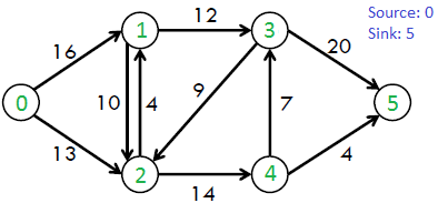
Maximum flow problems involve finding a feasible flow through a single-source, single-sink flow network that is maximum. Let's take an image to explain how the above definition wants to say.

👁 ford_fulkerson1

Each edge is labeled with capacity, the maximum amount of stuff that it can carry. The goal is to figure out how much stuff can be pushed from the vertex s(source) to the vertex t(sink). 

👁 ford_fulkerson2

maximum flow possible is : 23 

Following are different approaches to solve the problem :   

1. Naive Greedy Algorithm Approach (May not produce an optimal or correct result) Greedy approach to the maximum flow problem is to start with the all-zero flow and greedily produce flows with ever-higher value. The natural way to proceed from one to the next is to send more flow on some path from s to t How Greedy approach work to find the maximum flow :

E number of edge 
f(e) flow of edge 
C(e) capacity of edge 

1) Initialize : max_flow = 0 
 f(e) = 0 for every edge 'e' in E 

2) Repeat search for an s-t path P while it exists. 
 a) Find if there is a path from s to t using BFS
 or DFS. A path exists if f(e) < C(e) for 
 every edge e on the path.
 b) If no path found, return max_flow.
 c) Else find minimum edge value for path P

 // Our flow is limited by least remaining
 // capacity edge on path P.
 (i) flow = min(C(e)- f(e)) for path P ]
 max_flow += flow
 (ii) For all edge e of path increment flow 
 f(e) += flow

3) Return max_flow 

Note that the path search just needs to determine whether or not there is an s-t path in the subgraph of edges e with f(e) < C(e). This is easily done in linear time using BFS or DFS.

👁 image14

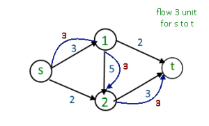
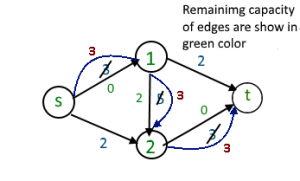
There is a path from source (s) to sink(t) [ s -> 1 -> 2 -> t] with maximum flow 3 unit ( path show in blue color ) 👁 image
👁 image

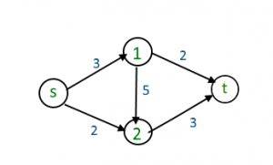
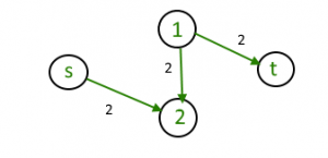
After removing all useless edge from graph it's look like

👁 maximum

For above graph there is no path from source to sink so maximum flow : 3 unit But maximum flow is 5 unit. to over come from this issue we use residual Graph.  

Below are the programs to implement the above concept:

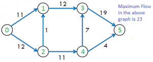
The maximum possible flow is 23

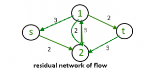
2. Residual Graphs

The idea is to extend the naive greedy algorithm by allowing “undo” operations. For example, from the point where this algorithm gets stuck in above image, we’d like to route two more units of flow along the edge (s, 2), then backward along the edge (1, 2), undoing 2 of the 3 units we routed the previous iteration, and finally along the edge (1,t) 👁 maximum

backward edge : ( f(e) ) and forward edge : ( C(e) - f(e) ) We need a way of formally specifying the allowable “undo” operations. This motivates the following simple but important definition, of a residual network. The idea is that, given a graph G and a flow f in it, we form a new flow network G_f that has the same vertex set of G and that has two edges for each edge of G. An edge e = (1,2) of G that carries flow f(e) and has capacity C(e) (for above image ) spawns a “forward edge” of G_f with capacity C(e)-f(e) (the room remaining) and a “backward edge” (2,1) of G_f with capacity f(e) (the amount of previously routed flow that can be undone). source(s)- sink(t) paths with f(e) < C(e) for all edges, as searched for by the naive greedy algorithm, corresponding to the special case of s-t paths of G_f that comprise only forward edges. 

The idea of residual graph is used The Ford-Fulkerson and Dinic's algorithms 

Source : http://theory.stanford.edu/~tim/w16/l/l1.pdf