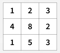
Given a 2D matrix cost[][], where each cell represents the cost of traversing through that position. We need to determine the minimum cost required to reach the bottom-right cell (m-1, n-1) starting from the top-left cell (0,0). The total cost of a path is the sum of all cell values along the path, including both the starting and ending positions. From any cell (i, j), you can move in the following three direction Right (i, j+1), Down (i+1, j) and Diagonal (i+1, j+1). Find the minimum cost path from (0,0) to (m-1, n-1), ensuring that movement constraints are followed.
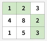
Output: 8 Explanation: The path with minimum cost is highlighted in the following figure. The path is (0, 0) -> (0, 1) -> (1, 2) -> (2, 2). The cost of the path is 8 (1 + 2 + 2 + 3).
[Naive Approach] Using Recursion - O(3 ^ (m * n)) Time and O(1) Space
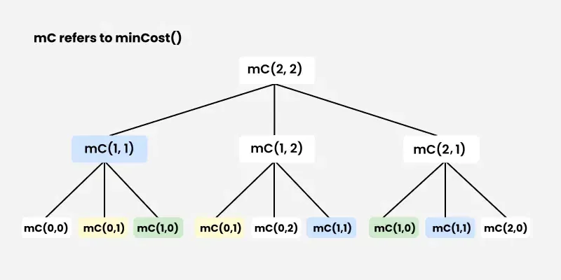
In this problem, we need to move from the starting cell (0,0) to the last cell (m-1, n-1). From every cell, we have three choices: we can move down (i+1, j), right (i, j+1), or diagonally (i+1, j+1). Whenever a problem gives multiple choices at every step, the first natural approach that comes to mind is recursion, because recursion allows us to break the problem into smaller independent subproblems.
To solve this using recursion, we start from the starting cell (0,0) and at each step we try all three possible moves. Each recursive call represents taking one of the paths, and since we want the minimum cost path, we simply try all possibilities and take the minimum among them. The base case occurs when the recursion reaches the last cell (m-1, n-1) - at that point, we stop and return the cost of that cell because the destination is reached.
Output
8
[Better Approach 1] Using Dijkstra's Algorithm - O((m * n) * log(m * n)) Time and O(m * n) Space
The idea is to apply Dijskra's Algorithm to find the minimum cost path from the top-left to the bottom-right corner of the grid. Each cell is treated as a node and each move between adjacent cells has a cost. We use a min-heap to always expand the least costly path first.
Output
8
[Better Approach - 2] Using Top-Down DP (Memoization) - O(m*n) Time and O(m*n) Space
If we look at the recursion tree, we notice that in recursion approach, many subproblems are solved again and again, which increases the time complexity. To handle this, we use a DP (memoization) approach. The idea is to store previously computed results in a DP table.
We create a 2D DP table of size (m × n) because there are two parameters that change in the recursive approach. After computing a subproblem, we store the result in the table. Later, when we encounter the same subproblem again, we check the table first. If the result is already computed, we return it instead of solving it again.
Output
8
[Better Approach - 3] - Using Bottom-Up DP (Tabulation) - O(m * n) Time and O(m * n) Space
In the previous approach, we used recursion along with memoization. Even though memoization helps us avoid recomputing the same subproblems, the recursive structure still makes the solution slower and harder to manage for large inputs. To make the solution more efficient, we switch to a bottom-up dynamic programming method, where we build the answer iteratively.
The idea is simple: we directly fill a DP table step by step. First, we set the base case:
dp[0][0] = cost[0][0], because the starting cell’s minimum cost is just its own value.
First row: Since movement is only from the left, dp[0][j] = dp[0][j - 1] + cost[0][j] (for j > 0)
First column: Since movement is only from above, dp[i][0] = dp[i - 1][0] + cost[i][0] (for i > 0)
Once these base cases are set, the remaining table can be filled using the main DP relation. For every cell (i, j), we consider the minimum cost among the three possible ways to reach it and add the current cell’s cost to that minimum. By filling the table in this order, we ensure that all required subproblems are already solved when we need them.
Output
8
[Expected Approach] - Using Space Optimized DP - O(m * n) Time and O(n) Space
In the previous approach, we used a 2D dp table to store the minimum cost at each cell. However, we can optimize the space complexity by observing that for calculating the current state, we only need the values from the previous row. Therefore, there is no need to store the entire dp table, and we can optimize the space to O(n) by only keeping track of the current and previous rows.
