Given a 2D array mat[][] of size n*m. The cost of a path is defined as the maximum absolute difference between the values of any two consecutive cells along that path. You are allowed to move up, down, left, or right to adjacent cells. Find the minimum possible cost of a path from (0, 0) to (n-1, m-1).
Examples:
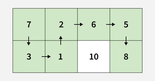
Input: mat[][] = [[7, 2, 6, 5], [3, 1, 10, 8]] Output: 4 Explanation: The route [7, 3, 1, 2, 6, 5, 8] has a minimum value of maximum absolute difference between two any consecutive cells in the route, i.e., 4.
The idea is to explore every possible path from the current cell to the destination using backtracking. At each step, we move in all valid directions and keep track of the maximum absolute difference between consecutive cell values along the current path. When we finally reach the destination, we compare the cost of this path with the global minimum and update the minimum cost if the current path offers a smaller value. To avoid revisiting cells within the same path, the current cell is temporarily marked as visited and restored afterward.
Output
4
Time complexity: 3(n*m), Since each of the m×n cells can branch into at most 3 new directions (excluding the previous cell), the overall time complexity is O(3^(m*n)). Auxiliary Space: O(n*m), stack space for a path from source to destination
[Better Approach] - Using Binary Search with Graph Traversal
The key idea is that the minimum possible maximum difference lies within a numeric range, so instead of checking all paths, we binary search on this value. For a given limit mid, we check whether a path exists from (0,0) to (n-1,m-1) such that every move satisfies:
abs(mat[next] - mat[curr]) ≤ mid
To verify this, we run a DFS/BFS and only move to neighbors that follow the limit. If the destination is reachable under this constraint, we try a smaller value; otherwise, we search higher.
Why we are not unmarking visited[][] array
We do not unmark visited cells because, for a fixed mid, DFS only needs to check whether a path exists (true/false), not compute any path value. When a cell is visited the first time, DFS explores all valid neighbors from it under the same mid condition. If a neighbor was already visited, its entire reachable area has already been checked, so revisiting it cannot lead to a different outcome.
Output
4
Time complexity: O((n*m) * log(k)), where k is max the values in the matrix, therefore, the maximum possible difference between the values of 2 consecutive cells can be k, hence the maximum cost can be k. And for each cost, we explore the grid, therefore the time complexity of exploring the grid is n*m Auxiliary Space: O(n*m)
[Expected Approach - 1] - Using Dijkstra's Algorithm
We can observe that along any path, the maximum difference so far never decreases—it either increases or stays the same. This property allows us to solve the problem using Dijkstra’s algorithm.
We treat each cell as a node, and edges connect adjacent cells with weights equal to the absolute difference of their values. We maintain a cost matrix where cost[i][j] is the minimum maximum difference needed to reach (i,j).
At each step, we process the cell with the current smallest cost and explore its neighbors. For each neighbor, the new cost is:
If newCost is smaller than the neighbor’s recorded cost, we update it.
When the destination is reached, its cost in the matrix gives the minimum possible maximum difference along any path.
Output
4
Time complexity: O((n*m) * log (n*m)), as the priority queue may contain n*m elements at max, and the cost of insertion/deletion of each element is log (size of priority queue). Auxiliary Space: O(n*m), the maximum size of priority queue
[Expected Approach - 2] - Using DSU - O((n*m) log(n*m)) Time and O(n*m) Space
We can treat each cell as a node and connect it to its neighbors with edges weighted by the absolute difference of their values. To represent each cell uniquely in DSU, we assign it a number using i*m + j, where i and j are the row and column indices and m is the number of columns.
We start connecting cells using the edges with the smallest differences first. Iteratively, we union the two cells of each edge. The moment the start (0, 0) and destination (n-1, m-1) become connected, the weight of the current edge is the minimum maximum difference along a path.
This works because by connecting edges from smallest to largest, the first time the start and end are connected ensures that the largest difference along the path is minimized, giving the correct answer.
