Program for Muller Method

Given a function f(x) on floating number x and three initial distinct guesses for root of the function, find the root of function. Here, f(x) can be an algebraic or transcendental function.
Examples: 
 

Input : A function f(x) = x + 2x + 10x - 20 and three initial guesses - 0, 1 and 2 .Output : The value of the root is 1.3688 or any other value within permittable deviation from the root. Input : A function f(x) = x - 5x + 2 and three initial guesses - 0, 1 and 2 .Output :The value of the root is 0.4021 or any other value within permittable deviation from the root. 

 

Muller Method

Muller Method is a root-finding algorithm for finding the root of a equation of the form, f(x)=0. It was discovered by David E. Muller in 1956.
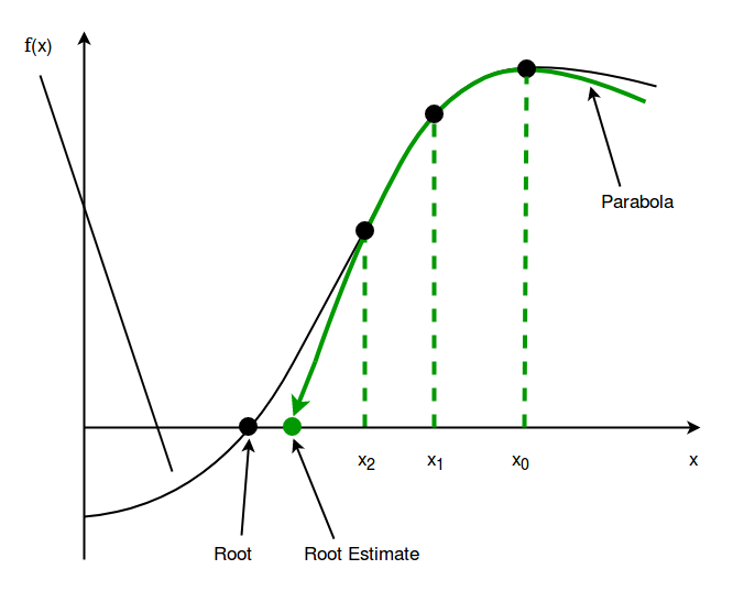
It begins with three initial assumptions of the root, and then constructing a parabola through these three points, and takes the intersection of the x-axis with the parabola to be the next approximation. This process continues until a root with the desired level of accuracy is found .
 

Why to learn Muller's Method?

Muller Method, being one of the root-finding method along with the other ones like Bisection Method, Regula - Falsi Method, Secant Method and Newton - Raphson Method. But, it offers certain advantages over these methods, as follows - 
 

1. The rate of convergence, i.e., how much closer we move to the root at each step, is approximately 1.84 in Muller Method, whereas it is 1.62 for secant method, and linear, i.e., 1 for both Regula - falsi Method and bisection method . So, Muller Method is faster than Bisection, Regula - Falsi and Secant method.
2. Although, it is slower than Newton - Raphson's Method, which has a rate of convergence of 2, but it overcomes one of the biggest drawbacks of Newton-Raphson Method, i.e., computation of derivative at each step. 
    

So, this shows that Muller Method is an efficient method in calculating root of the function.
 

Algorithm And Its Working

 

1. Assume any three distinct initial roots of the function, let it be x₀, x₁ and x₂. 
    
2. Now, draw a second degree polynomial, i.e., a parabola, through the values of function f(x) for these points - x₀, x₁ and x₂. 
   The equation of the parabola, p(x), through these points is as follows- 
   p(x) = c + b(x - x) + a(x - x), where a, b and c are constants.
    

👁 Image

1. 
    
2. After drawing the parabola, then find the intersection of this parabola with the x-axis, let us say x₃ . 
    
3. Finding the intersection of parabola with the x-axis, i.e., x₃: 
   
   • To find x, the root of p(x), where p(x) = c + b(x - x) + a(x - x), such that p(x) = c + b(x- x) + a(x- x)= 0, apply the quadratic formula to p(x).Since, there will be two roots, but we have to take that one which is closer to x.To avoid round-off errors due to subtraction of nearby equal numbers, use the following equation:
     
     Now, since, root of p(x) has to be closer to x, so we have to take that value which has a greater denominator out of the two values possible from the above equation.
   • To find a, b and c for the above equation, put x in p(x) as x, xand x, and let these values be p(x), p(x) and p(x), which are as follows-
     p(x) = c + b(x- x) + a(x- x)= f(x). 
     p(x) = c + b(x- x) + a(x- x)= f(x). 
     p(x) = c + b(x- x) + a(x- x)= c = f(x). 
      
   • So, we have three equations and three variables - a, b, c. After solving them to found out the values of these variables, we get the following values of a, b and c- 
      

c = p(x) = f(x) .b = (d*(h) - d*(h) ) / ( hh * (h - h)) .a = (d*(h) - d*(h)) / ( hh * (h - h)).

• 
  where, 
  d= p(x) - p(x) = f(x) - f(x) 
  d= p(x) - p(x) = f(x) - f(x) 
  h= x- x
  h= x- x
   
• Now, put these values in the expression for x- x, and obtain x. 
  This is how root of p(x) = xis obtained. 
   

1. If xis very close to xwithin the permittable error, then xbecomes the root of f(x), otherwise, keep repeating the process of finding the next x, with previous x, xand xas the new x, xand x. 
    

 

Output: 
 

The value of the root is 1.3688

Auxiliary Space: O(1)
Advantages 
 

• Can find imaginary roots.
• No need to find derivatives.

Disadvantages 
 

• Long to do by hand, more room for error.
• Extraneous roots can be found.

Reference- 
 

1. Higher Engineer Mathematics by B.S. Grewal.