Create a Gantt Chart in Google Sheets

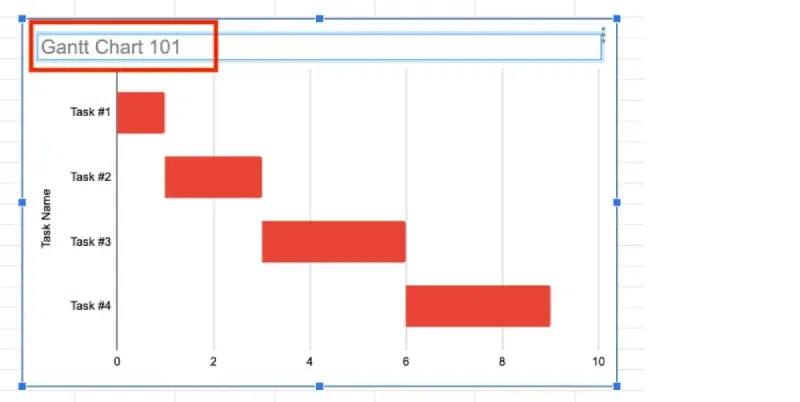
A Gantt chart in Google Sheets displays project tasks as bars along a timeline. Each bar shows the start, duration, and end dates of tasks, providing a clear overview of project progress. Its strength lies in tracking completed tasks, pending work, key milestones, expected outcomes, deliverables, and stakeholder responsibilities.

How to Make Gantt Chart in Google Sheets

Follow these easy steps to create a Gantt chart in Google Sheets:

Step 1: Open Google Sheets

After logging into Google, you will see nine dots at the top right corner. Click on it, and you will see the Google Sheets option while scrolling. Tap on it.

Step 2: Click on the Blank sheet

When entering Google Sheets, see the first option: Blank Sheet. Click on it.

Step 3: Input data into the Sheet

Enter your data in any cell of your choice.

For the first table, label the columns as follows:

• Column A: Task Name
• Column B: Start Date
• Column C: Duration

Then label the cells as follows:

• Cell A2: Task #1
• Cell A3: Task #2

Note:

Keep going until the Gantt chart has enough rows for every project job you wish to see. In addition to the header row, the table should include four rows if your project consists of four jobs, for instance.

Step 4: Add matching start and finish dates

Write starting and ending dates simultaneously, as shown in the image below.

Step 5: Make the second table

By creating it two or three rows below the first. In this instance, row 8 is where we begin the second table. Give the cells the following labels:

• Cell A8: Name of Task
• Cell B8: Begin on the Day
• Cell C8: Length

Step 6: Determine the Difference

Determine the difference between each task's start date (column B) and your project's initial task (probably in cell B2). This will indicate the days each job starts following the first one.

Step 7: Enter the Formula

In cell B9 (assuming your first task details start in row 2), type the following formula:

=int(B2)-int($B$2)

Note:

Explanation of the formulae

• The int() method ensures that the start day value is a whole number (days).
• B2: This refers to the cell (in our case) with the current task's start date.
• Hit the Enter key. Press Enter on your keyboard to finish.

Step 8: Use the same formula for each job in the Start on Day column

=int(B2) -int($B$2) To access the final project job, click cell B9 and then move the little blue Box located in the cell's bottom-right corner.

Step 9: Enter the following formula in the first cell

(C9) of the Duration column =(INT($B$4)-INT(C4))-(INT($B$4)-INT(B4) . On the keyboard, hit Enter. The value in the cell will automatically fill.

Note:

The cell numbers may change depending on where you put the project data in the sheet (for example, C4 may become C10), but the rest of the formula should stay the same.

Step 10: Use the following formula for each job in the Duration column:

=(INT($B$4)-INT(C4))-(INT($B$4)-INT(B4). After selecting cell C9, click and drag the little blue Box in the cell's lower-right corner to bring you to the final project assignment.

Step 11: Create a Bar Graph

Highlight the second table.

Step 12: Click Insert on the menu

Click on the insert option on the upper side of the sheet. Then click Chart underneath it. As you select it, a stacked bar chart appears on the page.

Step 13: Turn Your Stacked Bar Chart into a Gantt Chart

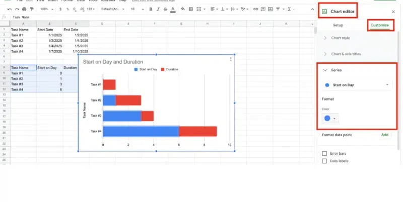
Click on any Start on Day bar in the Chart. This should highlight all the Start on Day bars.

Configure the Chart.

Step 14: Click the customizable Tab

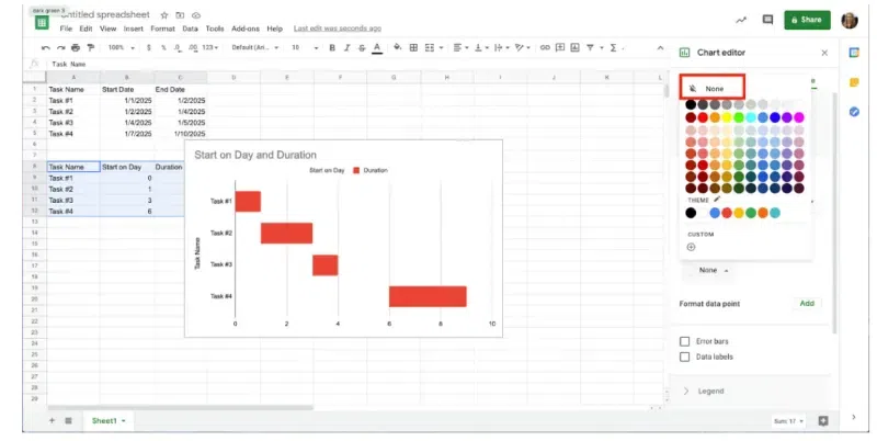
In the Chart editor panel on the right, click the Customize tab. Click Series, then click the dropdown menu and Start on Day. Click the Color button, then click None. The Chart should now resemble a Gantt chart.

How to Customize Your Gantt Chart in Google Sheets

Enhance the appearance of your Gantt chart by adjusting titles, colors, and styles to fit your project's needs. Follow the Steps to Customize your Gantt Chart in Google Sheets:

Step 1: Rename the Gantt chart

Double-click the Chart's title at the top. Enter a new project title here.

Step 2: Personalize the Gantt Chart Region

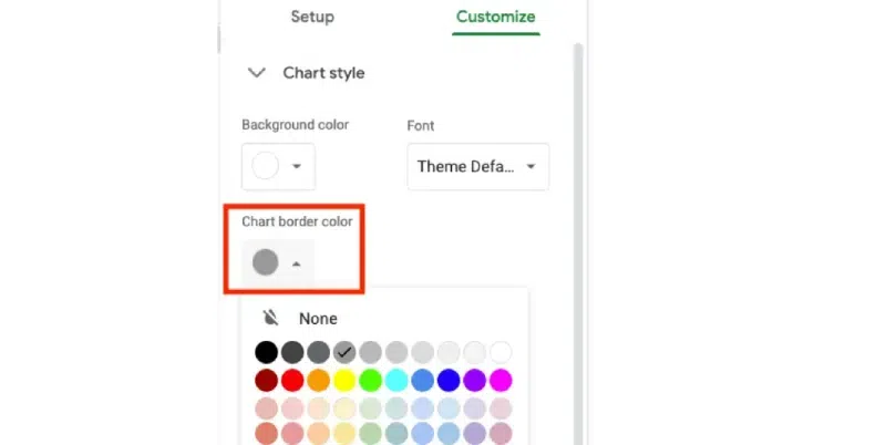
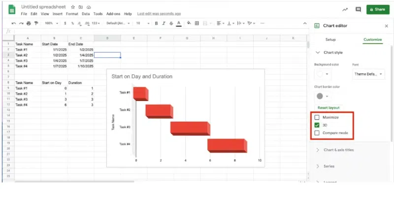
Make the bars stand out in three dimensions or change the border's colour.

Step 3: Go on chart editor

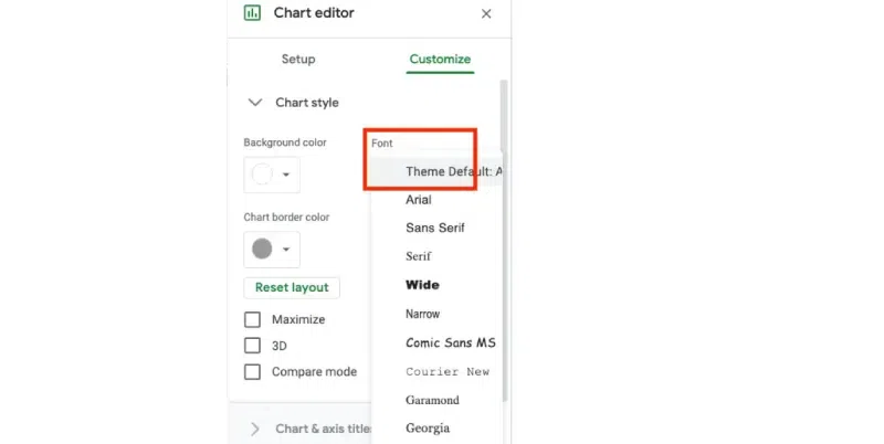
Click the Chart to access the Chart Editor menu on the right. After selecting the Customize tab, select the first choice, Chart style.

Step 4: Adjust the hue

Click the dropdown menu next to the Background colour and select a different colour.

Step 5: Alter the the text

To alter any text in the Chart, click on it. Use the Font dropdown menu to alter the font style for labels, legends, or the title.

Note:

To make changes, you will need to click on the text type.

Step 6: Visit "Chart border colour."

Click the dropdown menu labelled "Chart border colour." To entirely remove a border or colour, click None.

Step 7: Go to 3D Box

To apply the effect to the bars, click the 3D Box.

4. Free Gantt Chart Template for Google Sheets

To Access Free Gantt Chart in Google Sheets Follow the Below steps:

Step 1: Open Google Sheets

Step 2: Go to the Template Gallery and Scroll Down

Step 3: Select your Gantt Chart Template