How to Search and Find Data Efficiently in Google Sheets

Searching through large datasets in Google Sheets doesn't need to be a challenge. Whether you're handling financial records, tracking projects, or organizing data, efficient searching is key. In this article, you will learn how to search effectively in Google Sheets using various methods, including shortcuts, Find and Replace, and advanced functions. Master these techniques to streamline your workflow and enhance data management

1. How to Search in Google Sheets

There are two methods to search in Google Sheets. One is to use keyboard Shortcuts for Google Sheets learn and the other one is "Find and Replace" in Google Sheets. Read Below to learn the the both methods to search in Google Sheets.

• Method 1: Search in Google Sheet Using Keyboard Shortcuts.
• Method 2: Search in Google Sheet by Find and Replace method
• Method 3: Search in Google Sheet Using Conditional Formatting

2. Search in Google Sheets Using Keyboard Shortcuts

This shortcut is incredibly useful for locating specific data, especially in large spreadsheets. Learn 'how to search in Google sheet shortcut' below

Step 1: Press the Shortcut keys given below

Press CTRL + F (Windows) or CMD + F (Mac) together.

Step 2: See the search box in the right corner

A search box will appear in the top-right corner of your Google Sheets.

Step 3: Type the Text to search

Type the text you want to find within your spreadsheet.

Step 4: Google Sheet will highlight the searched text

Google Sheets will highlight the first occurrence of that text. Use the “Next” button to navigate through other instances of the same text.

Keyboard Shortcut to search in Google Sheet: CTRL + F (Windows) or CMD + F (Mac)

3. Search in Google Sheets Using Find and Replace

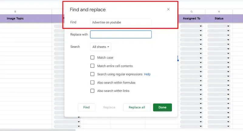
The “Find and Replace” feature is simple yet effective for locating and modifying data within your spreadsheet. Let’s explore how to use the “Find and Replace” feature in Google Sheets:

Step 1: Open your Google Sheets and click on the “Edit” menu at the top

Step 2: Choose "Find and replace" in the Edit menu

Choose the 'Find and Replace' option from the pop-up options.

Step 3: Type the term in the search box that appears

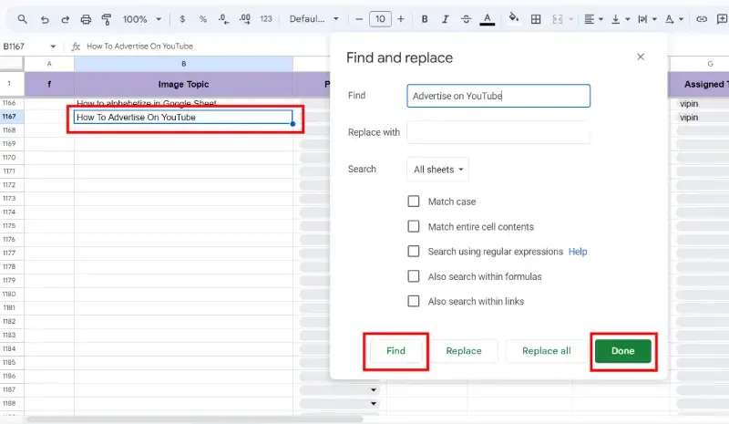
In the search box that appears, type the text you want to find within your spreadsheet. Google Sheets will locate the first occurrence of that text.

Step 4: Click on the “Options” button and Set Search Settings to Narrow Results

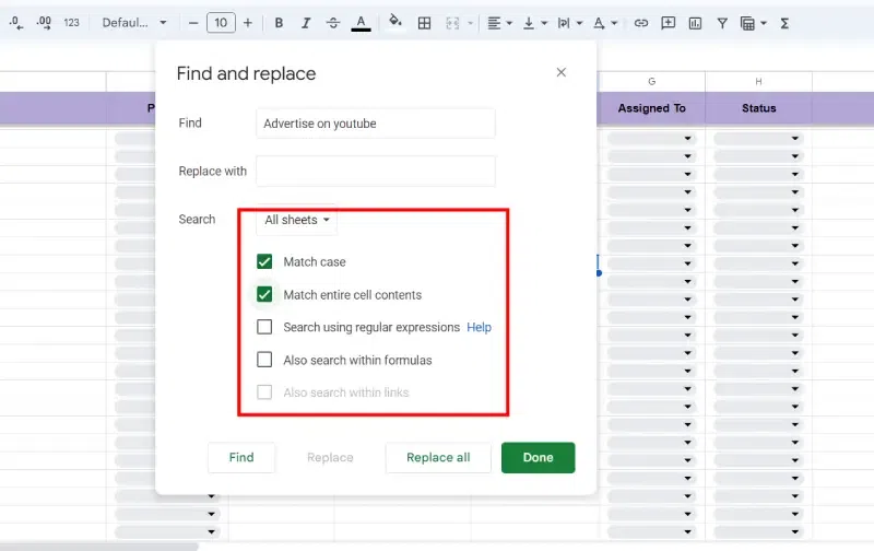
If you want to narrow down your search, click on the “Options” button. Here, you can specify additional criteria such as matching cases, whole words, or using regular expressions.

Step 5: Click “Find” or "Done" to See Multiple Results

Click the “Find” button to navigate through other instances of the same text. Google Sheets will highlight each occurrence as you proceed.

4. Search in Google Sheets Using Conditional Formatting

Conditional formatting can help highlight cells that meet certain criteria:

Step 1: Enter the data into the sheet

Input your data into the sheet.

Step 2: Drag to select the range of cells you want to search

Drag to select the range of cells you want to format.

Step 3: Go to Format and Select Conditional formatting from the menu

Navigate to Format and choose Conditional Formatting from the menu.

Step 3: Choose the formula

In the "Conditional format rules" sidebar that appears on the right, click the dropdown menu under "Format cells if" and select "Custom formula is" from the list of options.

Step 4: Preview Results

Set your conditions and apply formatting to highlight the results.

5. Google Sheets Search Functions

1. MATCH: This function helps find the position of a value within a range. It’s useful for locating specific data based on criteria.
2. INDEX: Use INDEX to retrieve values from a specified range. It’s handy for extracting data dynamically.
3. FIND: The FIND function locates the position of a substring within a text string. Great for searching within cell contents.
4. VLOOKUP: VLOOKUP searches for a value in the first column of a range and returns a corresponding value from another column. It’s powerful for cross-referencing data.

Also Read

• How to check for plagiarism on google docs