Google Sheets IF AND Function

The Google Sheets IF AND formula is a versatile tool that allows you to test multiple conditions at once and return specific results based on their outcomes. By combining logical functions, it helps streamline decision-making and automate tasks in data analysis. This feature is ideal for managing complex datasets, ensuring accuracy, and improving productivity in everyday spreadsheet work

How It Works:

The Google Sheets IF AND formula works by combining the logical AND function with the IF function to evaluate multiple conditions simultaneously. It checks if all specified conditions are true and then returns one value if they are true and another value if they are false.

• IF handles the decision-making: what happens if the condition is true or false?
• AND ensures that all the conditions being tested must be true for the formula to return the desired outcome.

Google Sheets IF AND Function Syntax

The syntax for using the IF AND function in Google Sheets is:

=IF(AND(condition1, condition2,), value_if_true, value_if_false)

Explanation:

• AND(condition1, condition2,): The AND function evaluates multiple logical conditions. It returns TRUE only if all the conditions are true.
• value_if_true: The result returned if all the conditions are true.
• value_if_false: The result returned if any condition is false.

1. How to Use The Google Sheets IF AND Function

You can use the Google Sheets IF AND by the following steps:

Step 1: Select a Cell

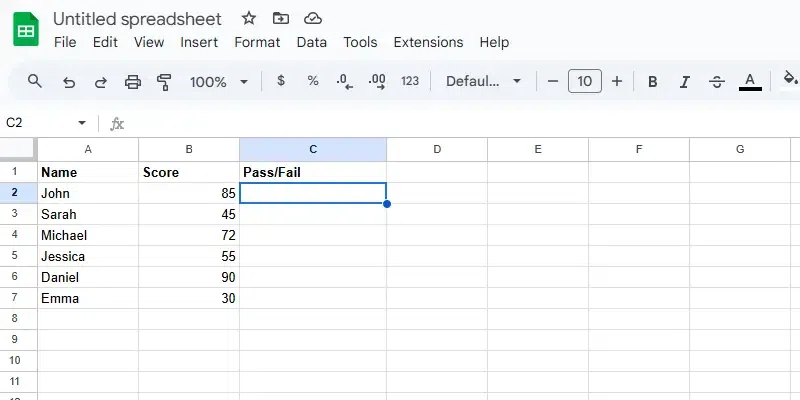
Click the cell where you want the result of the formula to appear. For example, select C2 to display the result for the first row of data.

Step 2: Enter the Formula

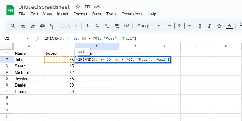
In the selected cell, type the following formula:

=IF(AND(B2 >= 50, B2 < 70), "Pass", "Fail")

This formula checks if the score in column B (Score) is greater than or equal to 50 but less than 70. If both conditions are true, the student will be marked as "Pass", otherwise "Fail".

• Condition 1: B2 >= 50 checks if the score is 50 or more.
• Condition 2: B2 < 70 checks if the score is less than 70.

Example Formula Breakdown:

• AND(B2 >= 50, B2 < 70) checks if the score is between 50 and 69.
• If both conditions are true, it returns "Pass"; otherwise, it returns "Fail".

For example, if:

• B2 = 85, the formula will return "Pass" (since 85 >= 50 and 85 < 70).
• B2 = 45, the formula will return "Fail" (since 45 is not >= 50).
• B2 = 72, the formula will return "Fail" (since 72 is not < 70).

Step 3: Press Enter

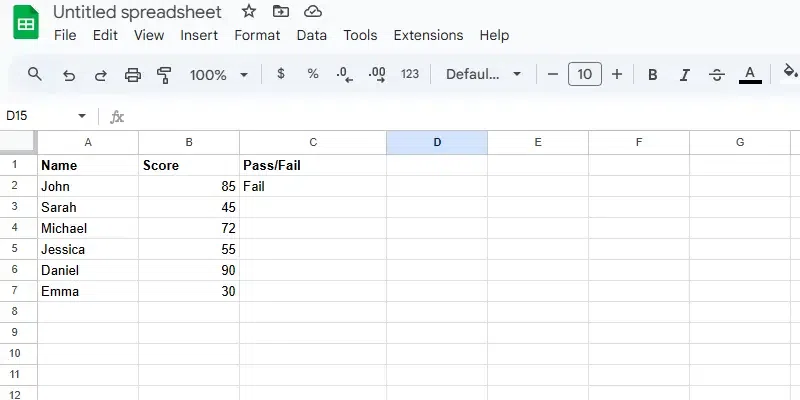
After typing the formula, press Enter to apply the formula. The cell will now display the result based on the conditions you set.

Step 4: Apply the Formula to Other Rows

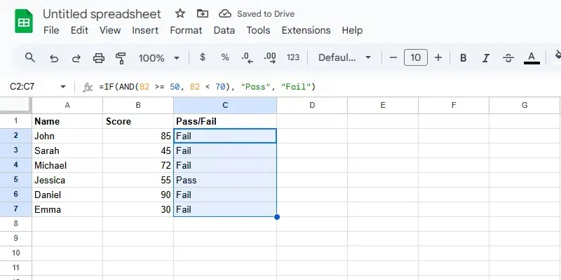
Once the formula is working for the first row, you can apply it to the rest of the rows:

• Click the lower-right corner of the formula cell (C2) until you see a small square handle.
• Drag the handle down to fill the formula in the remaining cells in column C.

Final Notes:

• This formula uses AND to evaluate if the score meets both conditions (50 ≤ score < 70).
• You can modify the formula to include different conditions as needed. For example, you could check if the score is above 70 for a "Pass" result by adjusting the conditions.

Also Read:

• How to Highlight Duplicates in Google Sheets
• How to Create a Digital Planner in Google Sheets
• How to Change Cell Height and Width in Google Sheets