 |
VOOZH | about |
|
VOOZH | about |
The IFS function in Google Sheets evaluates multiple conditions and returns the value corresponding to the first true condition. It's particularly useful when you need to check several conditions without nesting multiple IF functions. The IFS function simplifies your formulas and makes your data management tasks more efficient.
The syntax for the IFS function is as follows:
IFS(condition1, value1, condition2, value2, condition_n, value_n)
You can include as many conditions and true values as needed.
To use the IFS Function in Google Sheets follow the steps given below:
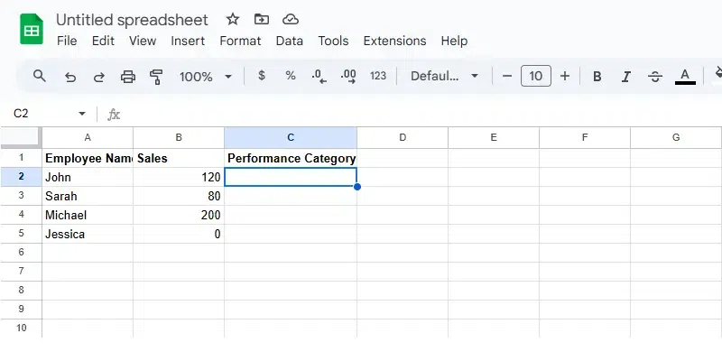
Start by opening your Google Sheets document where you want to use the IFS function.
Click on the cell where you want the result of the formula to appear. For this example, click on C2 in the "Performance Category" column.
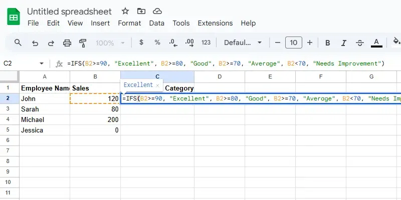
Type or paste the IFS formula in the selected cell. Here's an example:
=IFS(B2>=90, "Excellent", B2>=80, "Good", B2>=70, "Average", B2<70, "Needs Improvement")
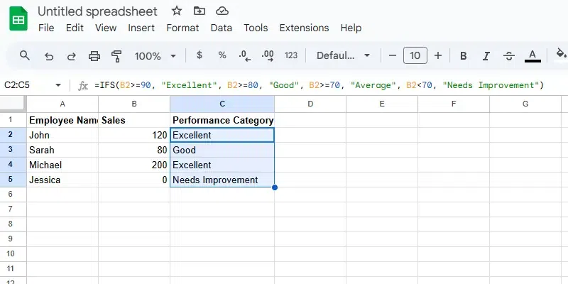
B2 >= 90 assigns "Excellent" if the sales are 90 or more.B2 >= 80 assigns "Good" if the sales are between 80 and 89.B2 >= 70 assigns "Average" if the sales are between 70 and 79.B2 < 70 assigns "Needs Improvement" if the sales are below 70.After typing the formula, press Enter to apply it. The cell will display the performance category based on the sales data.
To apply the formula to other rows:
Notes:
- The IFS function evaluates conditions in order, returning the result for the first condition that is true.
- Ensure that the conditions are arranged in descending order so that the function checks the higher values first.
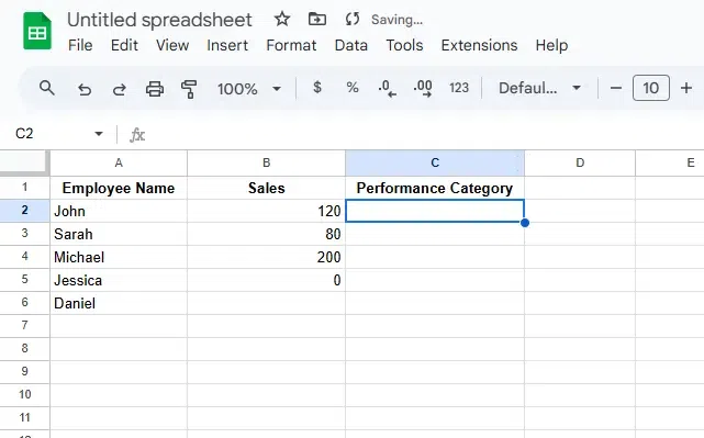
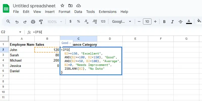
The Advanced IFS Function in Google Sheets allows you to handle multiple conditions, including blanks and special cases. This is useful when you want to evaluate different criteria in a more flexible and efficient way. Below are the steps for applying the advanced IFS formula to the given data:
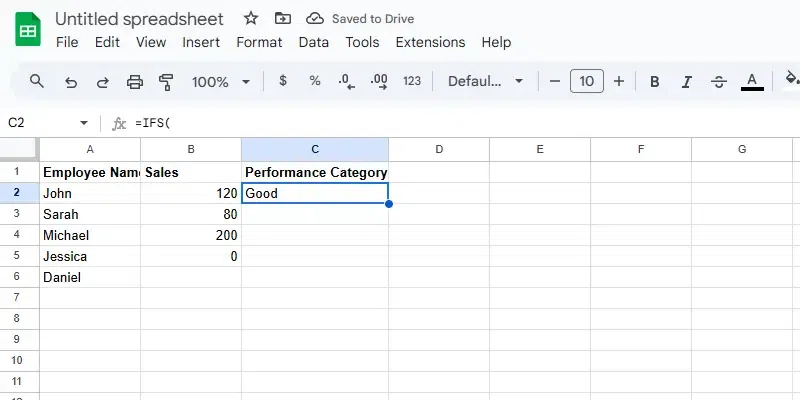
Click on the cell where you want the result to appear. For example, click on C2 in the "Performance Category" column, as this is where the performance result will be displayed.
In the selected cell (C2), type or paste the following IFS formula:
=IFS(
B2>=150, "Excellent",
AND(B2>=100, B2<150), "Good",
AND(B2>=50, B2<100), "Average",
B2=0, "Needs Improvement",
ISBLANK(B2), "No Data"
)
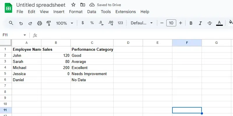
B2 >= 150 returns "Excellent" if the sales are 150 or more.AND(B2 >= 100, B2 < 150) returns "Good" if the sales are between 100 and 149.AND(B2 >= 50, B2 < 100) returns "Average" if the sales are between 50 and 99.B2 = 0 returns "Needs Improvement" if the sales are 0.ISBLANK(B2) returns "No Data" if the sales cell (B2) is blank.After typing the formula, press Enter to apply it. The cell will display the performance category based on the sales value in B2.
To apply the formula to other rows:
Notes:
- The IFS function evaluates conditions in order, returning the result for the first condition that is true.
- Using the
ANDfunction allows you to combine multiple conditions within a single formula.- The
ISBLANKfunction helps handle blank cells, making the formula more dynamic.
You can use the IFS function to categorize numerical data into specific ranges. For example, classifying students' scores into grades (A, B, C) based on their performance.
Example:
=IFS(A2 >= 90, "A", A2 >= 80, "B", A2 >= 70, "C", A2 < 70, "F")
This formula assigns letter grades based on the value in cell A2.
The IFS function can be paired with conditional formatting to automatically change cell colors based on certain conditions. For example, you can color code sales performance (excellent, good, poor) in your sales report.
The IFS function eliminates the need for nested IF functions, making it easier to manage multiple conditions. For instance, if you need to test multiple eligibility criteria, you can use the IFS function instead of writing several IF statements.