Google Sheets LEFT Function

The LEFT function in Google Sheets is a simple tool that allows you to extract a specific number of characters from the beginning of a text string. Whether you're working with addresses, names, or product codes, the LEFT function makes it easy to isolate the beginning portion of the text. This function is particularly useful when you're dealing with standardized data or need to break down a larger dataset into more manageable parts.

1. Google Sheets LEFT Function

The LEFT function in Google Sheets extracts a specific number of characters from the beginning (left side) of a text string. It's a handy tool for separating or analyzing text data, such as pulling prefixes, codes, or initials from larger strings.

How It Works

The LEFT function takes a text input and a number as arguments. It returns the first specified number of characters from the text, starting from the left. This function is commonly used for tasks like extracting abbreviations or trimming text for further analysis.

Google Sheets LEFT Function Syntax

Here is the syntax of the LEFT function in Google Sheets:

=LEFT(text, [number_of_characters])

• text: The text string or cell reference from which you want to extract characters.
• number_of_characters (optional): The number of characters you want to extract from the left. If omitted, the function returns just one character.

The LEFT function is simple to use and helps in managing text-based data efficiently.

2. How to Use the LEFT formula in Google Sheets

Follow the steps given below to use LEFT Function in Google Sheets:

Step 1: Select the Cell for the Result

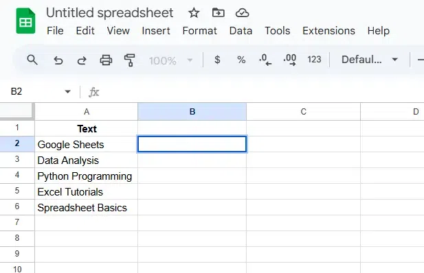
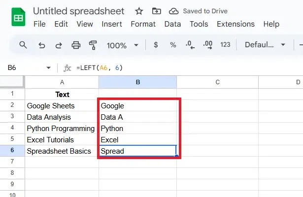
Choose the cell where you want the extracted text to appear. For example, select B2.

Step 2: Identify the Cell with Text

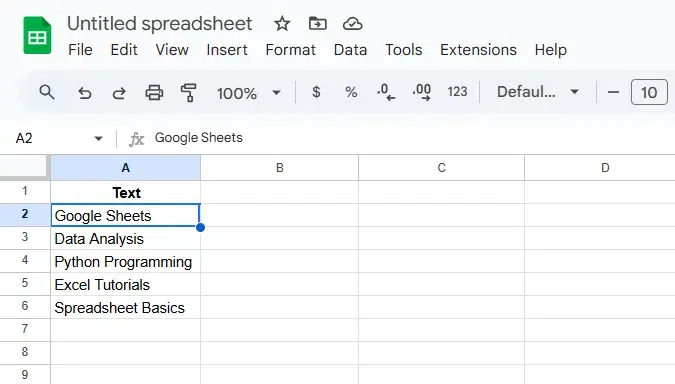
Locate the cell containing the text you want to extract from. For instance, A2 with the text "Google Sheets".

Step 3: Insert the LEFT Formula

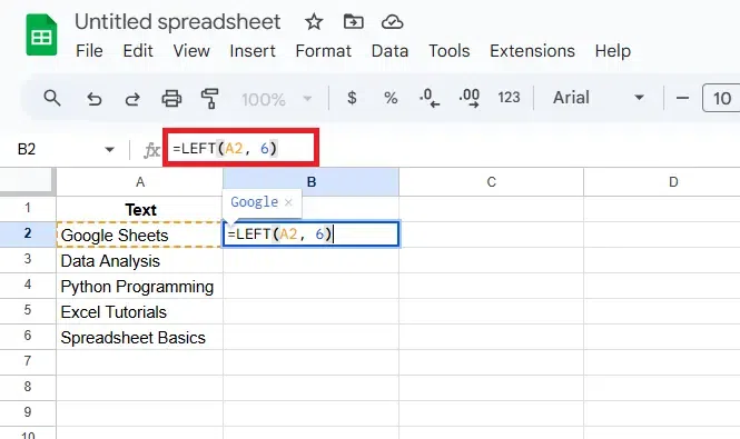
In the selected cell (B2), type the formula:

=LEFT(A2, 6)

This extracts the first 6 characters from the text in A2, which would result in "Google".

Step 4: Press Enter

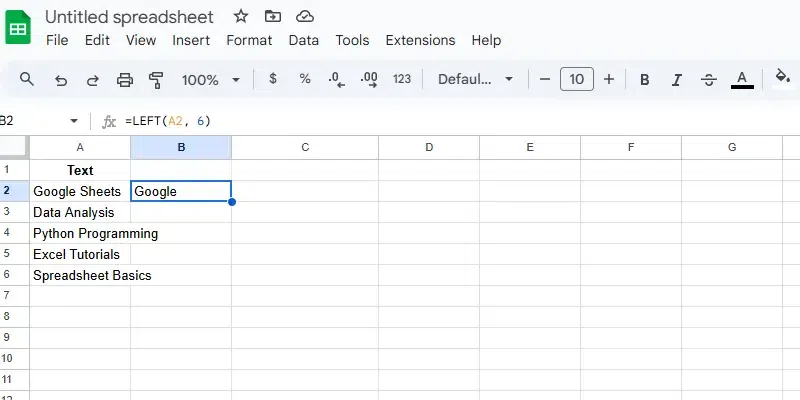
Hit Enter to apply the formula. The result, "Google", will be displayed in B2.

Step 5: Apply Formula to Other Cells (Optional)

If you want to apply the same formula to other cells in the column, simply drag the fill handle (the small square at the bottom right corner of B2) down to the desired cells.

3. Using LEFT with FIND Function in Google Sheets

Here we will combine the LEFT function with the FIND function to dynamically extract text up to a specific character or word.

Step 1: Select the Cell for the Result

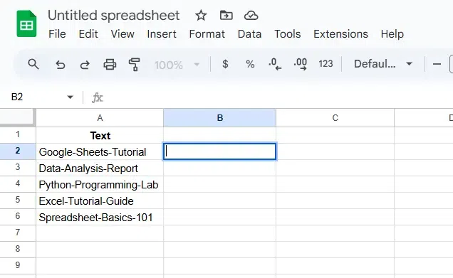
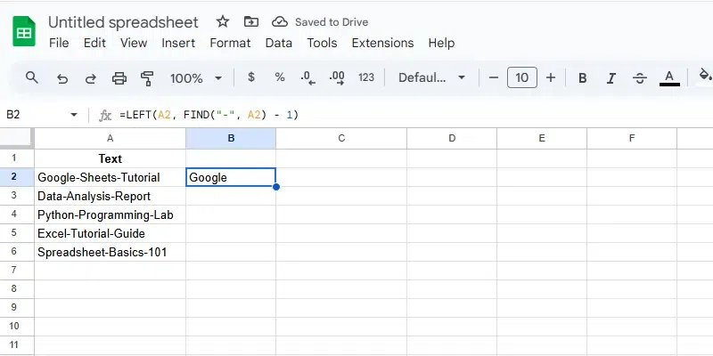
Choose the cell where you want the extracted text to appear. For example, select B2.

Step 2: Identify the Cell with Text

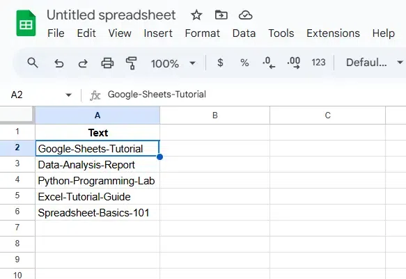
Locate the cell containing the text you want to extract from. For example, A2 contains the text "Google-Sheets-Tutorial".

Step 3: Insert the LEFT with FIND Formula

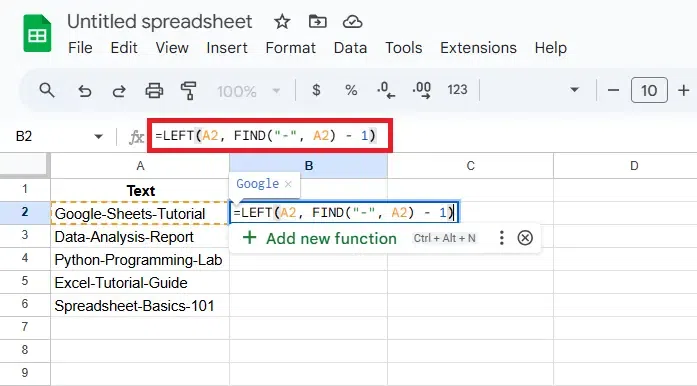
In the selected cell (B2), type the formula:

=LEFT(A2, FIND("-", A2) - 1)

This formula performs two actions:

• FIND("-", A2) locates the position of the first hyphen ("-") in the text in A2.
• LEFT(A2, FIND("-", A2) - 1) extracts all text to the left of the hyphen (but not including the hyphen itself). In this case, the result will be "Google".

Step 4: Press Enter

Hit Enter to apply the formula. The result in B2 will be "Google".

Step 5: Apply the Formula to Other Rows (Optional)

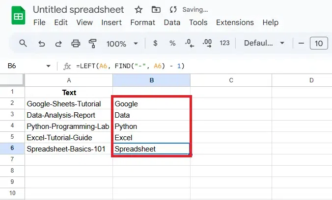
If you want to extract text for other rows, drag the fill handle (the small square at the bottom right corner of B2) down to the other cells (e.g., B3:B6). The formula will adjust automatically for each row, extracting text up to the first hyphen in the corresponding cell in column A.

Also Read:

• SUMIF in Google Sheets with formula examples
• How to Lock Cells in Google Sheets
• How to Automate Task in Google Sheets