How to Use VLOOKUP in Google Sheets

The VLOOKUP formula stands for Vertical Lookup. It searches a specific value (known as the search key) in the first column of a defined range and returns a corresponding value from another column in the same row.

This function is essential for retrieving values across rows where data is structured in vertical columns.

VLOOKUP Syntax:

=VLOOKUP(search_key, range, index, [is_sorted])

Parameters:

• search_key: The value you're looking for (e.g., product name or ID).
• range: The table or range where the data exists.
• index: The column number (starting from 1) of the value to return.
• is_sorted(optional): FALSE for exact matches (recommended), TRUE for approximate.

1. How to use VLOOKUP in Google Sheets

Here are the steps to use VLOOKUP in Google Sheets, along with some helpful VLOOKUP formula examples in Google Sheets to guide you:

Step 1: Organize Your Data

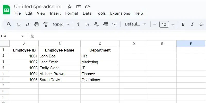
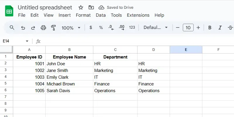
Ensure that your data is structured with the Employee ID in the first column (Column A), the Employee Name in the second column (Column B), and the Department in the third column (Column C).

Step 2: Choose the Cell for the Formula

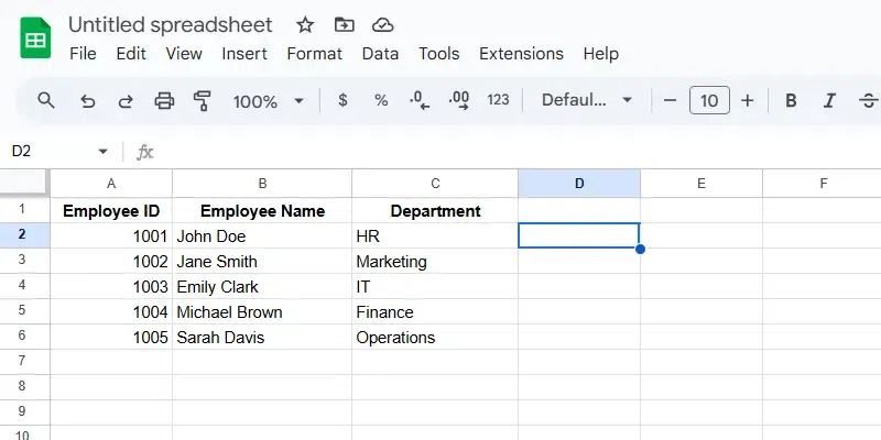
Decide where you want the result of the VLOOKUP formula to appear. Let's assume you want the Department to appear in Cell D2 when you enter an Employee ID in Cell A2.

Step 3: Enter the VLOOKUP Formula

In Cell D2, use the following formula to search for the Employee ID in Column A and retrieve the corresponding Department from Column C.

Formula:

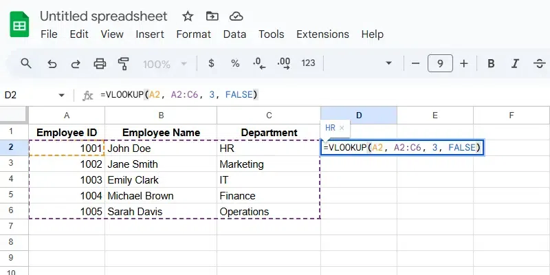
=VLOOKUP(A2, A2:C6, 3, FALSE)

Here’s the breakdown:

• A2: The lookup value — the Employee ID (e.g., "1001").
• A2:C6: The range where the lookup value will be searched (including Employee IDs, Employee Names, and Departments).
• 3: The column index (Department is in the third column of the range).
• FALSE: This ensures that you are looking for an exact match of the Employee ID.

Step 4: Press Enter

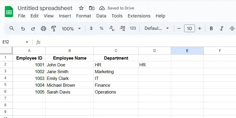
After entering the formula in Cell D2, press Enter. The Department corresponding to the Employee ID in A2 will appear in D2.

For example, if you type "1001" in A2, D2 will display "HR".

Step 5: Drag the Formula to Other Cells

To apply the formula to other rows, click on the small square in the bottom-right corner of Cell D2 (the fill handle) and drag it down to the other cells in Column D.

For example, typing "1002" in A3 will return "Marketing" in D3, and so on.

Key Points:

• The Employee ID is the lookup value (in Column A).
• Department is the value we want to retrieve (from Column C).
• We used the VLOOKUP function to search for the Employee ID and return the Department.
• False ensures that only an exact match will return a result.

This example shows how to use VLOOKUP to search for an Employee ID and retrieve the corresponding Department from a dataset.

2. How to Use VLOOKUP from Another Sheet in Google Sheets

To VLOOKUP data from a different sheet in Google Sheets, you'll need to reference the data from one sheet while using a formula in another. This can be useful when you're working with large datasets that are split across multiple sheets, and you want to retrieve information based on a lookup value.

Step 1: Prepare Your Sheets

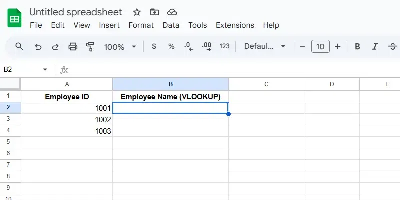
Make sure the data is spread across two sheets. For example:

Sheet1: Contains the formula you will use to retrieve data.

Sheet2: Contains the data you want to search from.

Step 2: Identify the Lookup Value and Range

Determine the lookup value and the range where the value is located.

For example:

• Sheet1 (the formula sheet): Column A will have the Employee ID that you will search for.
• Sheet2 (the data sheet): Column A contains the Employee ID, and Column B contains the Employee Name.

Step 3: Write the VLOOKUP Formula

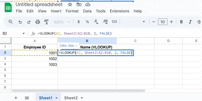
In the cell where you want the result (in Sheet1), use the following VLOOKUP formula:

=VLOOKUP(A2, Sheet2!A2:B10, 2, FALSE)

Here’s what each part means:

A2: The lookup value (Employee ID in Sheet1).

• Sheet2!A2:B10: The range where the Employee IDs and Names are located (in Sheet2).
• Sheet2! tells Google Sheets that the range is on a different sheet.
• A2:B10 refers to the range containing Employee IDs (Column A) and Employee Names (Column B) in Sheet2.

2: The column index number. Since Employee Name is in the second column of the range (Column B), we use 2.

• FALSE: This ensures that the formula looks for an exact match for the Employee ID.

Step 4: Press Enter

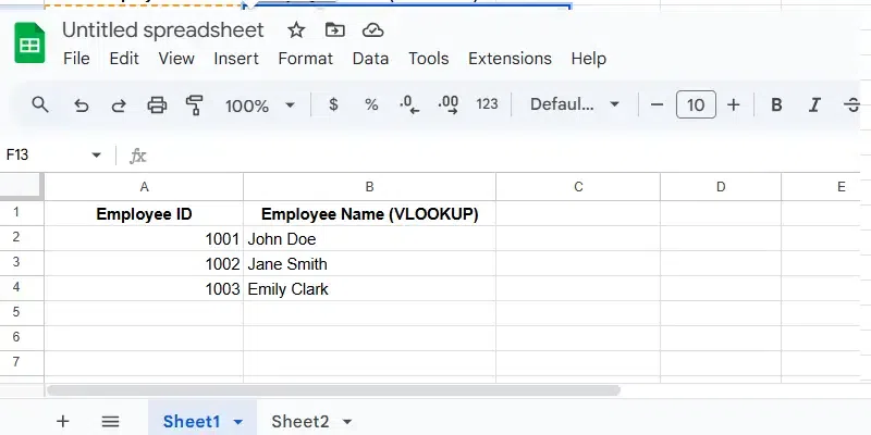
Press Enter to apply the formula. The cell in Sheet1 will now display the corresponding Employee Name from Sheet2 based on the Employee ID in A2 of Sheet1.

Step 5: Drag the Formula to Other Cells (Optional)

If you want to apply the formula to other rows, click on the small square in the bottom-right corner of the cell containing the formula (the fill handle) and drag it down to the other cells. This will automatically adjust the formula to lookup the values in the new rows.

Key Points to Remember:

• When you reference a different sheet, use the format SheetName!Range. For example: Sheet2!A2:B10.
• Ensure you use the correct range and column index in the formula.
• FALSE is important for finding an exact match. If you use TRUE, it looks for an approximate match (sorted data).

3. How to VLOOKUP With Wildcard in Google Sheets

Using VLOOKUP with Wildcard Characters in Google Sheets allows you to search for partial matches or patterns within your data. Wildcards help when you don’t need to match an exact value but rather a part of the value, giving you flexibility in your search.

3.1. What are Wildcard Characters?

• Asterisk (*): Represents any number of characters (including zero characters).
• Question Mark (?): Represents a single character.

Example Scenario

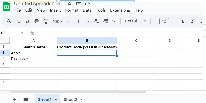
Suppose you have a list of product names and their corresponding product codes, and you want to search for products containing a certain keyword (e.g., "Apple") in their names. By using wildcards, you can search for product names that include the word "Apple" anywhere in the text.

Sheet1 (Lookup Table):

Sheet2 (Data Table):

Step 1: Prepare Your Data

Ensure your data is organized properly across two columns—one containing the lookup values and another containing the results. Let’s use the following sample dataset:

Step 2: Identify the Lookup Value and Range

You need to know what value you want to search for and where to search it.

• Lookup Value: Let’s say we want to search for products that contain the word “Apple”.
• Range: Your data range is in Sheet2!B2:C6, where B2:B6 contains the Product Names and C2:C6 contains the Product Codes.

Step 3: Write the VLOOKUP Formula with Wildcard Characters

The VLOOKUP function can be combined with wildcards for partial matching.

• Search for products that contain the word “Apple” anywhere in their names:

Formula:

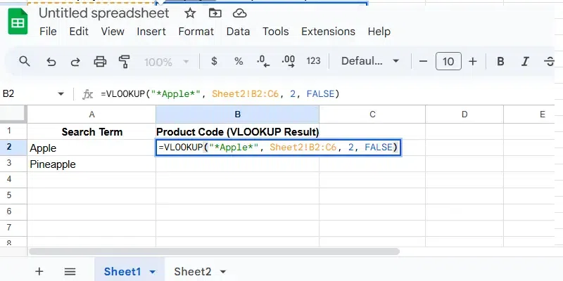
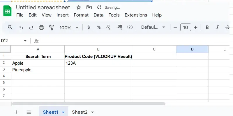
=VLOOKUP("*Apple*", Sheet2!B2:C6, 2, FALSE)

Explanation:

• "*Apple*": The * wildcard allows you to match any characters before or after "Apple". This means it will match "Apple Juice", "Apple and Mango", or any other product name containing the word "Apple".
• Sheet2!B2:C6: This is the data range where we are searching (Product Names in column B and Product Codes in column C).
• 2: This is the column index from which the result will be returned. Here, column 2 is where the Product Code is located.
• FALSE: This ensures the match is exact, considering the wildcard.

Step 4: Press Enter

Once you enter the formula in the desired cell (for example, in Sheet1!B2), press Enter. The formula will return the Product Code of the first matching result. In this case, it will return the code for "Apple Juice" (i.e., 123A).

Step 5: Apply to Other Cells (Optional)

If you want to search for other keywords or apply the same formula to more rows, drag the formula down. This will adjust the cell references accordingly and perform the search for the new values.

4. How to Use a Case Sensitive VLOOKUP in Google Sheets

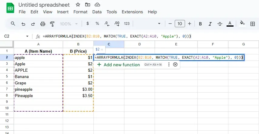
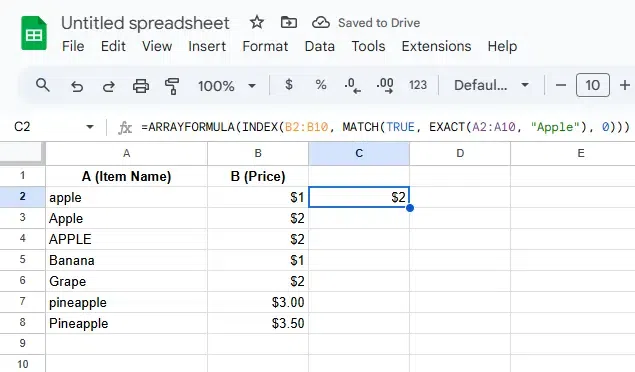
By default, VLOOKUP in Google Sheets isn’t case-sensitive, which means it treats "apple" and "Apple" as the same. To make it case-sensitive, you can use a combination of functions like ARRAYFORMULA, INDEX, and MATCHto customize your lookup. This method ensures that the function distinguishes between uppercase and lowercase letters.

Step 1: Use an Array Formula for Case-Sensitive Lookup

You can use the following formula to perform a case-sensitive lookup in Google Sheets:

=ARRAYFORMULA(INDEX(B2:B10, MATCH(TRUE, EXACT(A2:A10, "Apple"), 0)))

Breakdown of the Formula:

• EXACT(A2:A10, "Apple"): This part of the formula checks if each cell in the range A2:A10 exactly matches the case-sensitive text "Apple". The EXACT function ensures that "apple" and "Apple" are treated as different values.
• MATCH(TRUE, EXACT(A2:A10, "Apple"), 0): The MATCH function looks for the first occurrence of TRUE (i.e., an exact match) in the array generated by the EXACT function. It returns the relative position of the matching value within the range A2:A10.
• INDEX(B2:B10, ): Once MATCH finds the position of the case-sensitive match, the INDEX function returns the corresponding value from column B2:B10.
• ARRAYFORMULA: This allows the formula to process entire arrays (ranges) at once, enabling it to evaluate the entire range A2:A10 and find the exact match.

Step 2: Press Enter

After entering the formula in the desired cell (for example, C2), press Enter. The formula will return the value from column B2:B10 that corresponds to the case-sensitive match in column A2:A10.

5. Best Practices for Using VLOOKUP

• Always set is_sorted to FALSE for exact matches.
• Use named ranges for easier readability.
• Combine with IFNA or IFERROR to avoid broken outputs.
• Format data consistently (no extra spaces, consistent data types).

6. VLOOKUP vs INDEX-MATCH

7. VLOOKUP Not Working : Troubleshooting VLOOKUP Errors

Using the VLOOKUP function in Google Sheets can sometimes result in errors, which can be frustrating. Below are common VLOOKUP errors and how to troubleshoot them:

1. #N/A Error

Cause: The function cannot find the lookup value in the first column of the range.

Solutions:

• Double-check the lookup value for typos or inconsistencies.
• Ensure the lookup value exists in the first column of the range.
• Verify that the lookup type (exact or approximate match) is appropriate.

2. #REF! Error

Cause: The column index number exceeds the number of columns in the lookup range.

Solutions:

• Revisit the col_index_num argument to ensure it falls within the range's column count.
• Expand the range if more columns need to be included.

3. #VALUE! Error

Cause: Non-numeric values are used where numeric ones are expected.

Solutions:

• Check the column index number to ensure it’s a positive integer.
• Verify that all referenced cells contain compatible data types.

4. #DIV/0! Error

Cause: The function attempts to divide by zero during calculations within the range.

Solutions:

• Look for blank or zero-value cells in your range.
• Replace zero values or update the formula to handle empty cells.

5. Incorrect Results

Cause: VLOOKUP might return unexpected results when the lookup is not sorted or if duplicates exist.

Solutions:

• For approximate matches (TRUE as the fourth argument), ensure the first column is sorted in ascending order.
• Remove or handle duplicate entries in the lookup column.

6. Case-Sensitivity Issues

Cause: VLOOKUP is not case-sensitive, leading to potential mismatches.

Solutions:

• Use array formulas or helper columns for case-sensitive lookups.

8. General Tips to Avoid Errors:

• Check Data Format: Ensure consistent formatting (e.g., text, numbers) in the lookup column.
• Use Exact Matches: Set the fourth argument to FALSE for more precise results.
• Leverage IFERROR: Wrap the VLOOKUP formula with IFERROR to handle errors gracefully:

  =IFERROR(VLOOKUP(A1, B1:D10, 2, FALSE), "Not Found")

By addressing these common issues, you can effectively troubleshoot and resolve VLOOKUP errors in Google Sheets.