How to Use Conditional Formatting in Google Sheets

Conditional formatting in Google Sheets is a tool that automatically styles cells based on specific rules, making it easier to highlight trends, identify outliers, or emphasize critical data. Whether you're managing budgets, tracking project milestones, or analyzing sales data, conditional formatting enhances data visualization and decision-making.

Conditional Formatting in Google Sheets

Conditional formatting dynamically styles cells based on predefined conditions or custom formulas. It allows you to:

• Highlight specific text, numbers, or dates.
• Color-code cells based on their values.
• Apply formatting to entire rows or ranges.
• Use custom formulas for complex logic, such as identifying errors or time-based conditions.

For example, you can highlight sales above $500 in green or flag overdue tasks in red, making data insights instantly actionable.

How to Apply Conditional Formatting in Google Sheets

Follow these steps to apply conditional formatting in Google Sheets:

Prerequisites

• Open Google Sheets via Google Workspace (access through the 9-dot menu in your browser or directly at sheets.google.com).
• Use a spreadsheet with data or create a new one.

How to use Conditional Formatting in Google Sheets

Google Sheets' conditional formatting automatically styles cells according to present criteria, enhancing the platform's functionality. The steps to how to use:

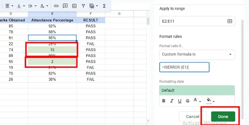
Step 1: Select the Range

Choose the Range of cells for conditional formatting.

Step 2: Go to the format menu and Select Conditional Formatting

Go to the format menu and select conditional formatting

Step 3: Add a new rule

Click "Add new rule" in the Conditional format rules pane.

Step 4: Set Condition

Select conditions like more significant than, less than, equal to, etc.

Step 5: Choose Formatting

Select cell formatting when the condition is met. Options include text and background colours, borders, etc.

Step 6: Press Done to apply

To apply the changes, press the done button

Step 7: Preview Results

The formatted cells will update automatically with changing conditions.

How to Apply Conditional Formatting with is empty/is not empty

Step 1: Select the Range

Select the Range of the cell in Google Sheets.

Step 2: Open Conditional Formatting

Click on the "Format" menu and select "Conditional formatting."

Step 3: Add New Rule

Click "Add new rule" in the Conditional format rules.

Step 4: Choose a Condition from the Format rules

Go to the Format rules, and Select "Custom formula is."

Step 5: Enter the Formula

Enter Formula, and define the "= ISBLANK (C1)" and "=NOT(ISBLANK(C1)" formulas.

Step 6: Choose Style

Set Formatting style in google sheet.

Step 7: Select the Done option

To apply the changes, press the done button.

How to Apply Conditional Formatting based on Text

Step 1: Select the Range

Select the Range of the cell in Google Sheets.

Step 2: Open Conditional Formatting

Go to the format menu and select conditional formatting

Step 3: Add a new rule

Click "Add new rule" in the Conditional format rules pane.

Step 4: Choose a Condition from the dropdown menu

Under "Format cells if...", you can select "Text contains, Text does not contain, Text is exactly or another relevant option.

Step 5: Enter Text

Input the condition text (e.g., "PASS OR FAIL").

Step 6: Set Formatting

The select style for cells when the condition is met (e.g., text color, background).

Step 7: Press Done to apply

Click "Done" to apply conditional formatting.

How to Apply Conditional Formatting based on number values

Step 1: Select the Range

Select the Range of the cell in Google Sheets.

Step 2: Open Conditional Formatting

Go to the format menu and select conditional formatting

Step 3: Add a new rule

Click "Add new rule" in the Conditional format rules pane.

Step 4: Choose Condition

In the Conditional Formatting menu, select a condition, such as "Greater Than" or "Less Than."

Step 5: Set the VALUE and Click Done Button

Specify a value after choosing the condition and Apply the rule by clicking "Done".

How to Apply Conditional Formatting to an Entire Row

Step 1: Select the Range

Select the Range of the cell in Google Sheets.

Step 2: Open Conditional Formatting

Go to the format menu and select conditional formatting

Step 3: Choose Condition

In the Conditional formatting rules pane, choose "Custom formula."

Step 4: Enter Formula "= $A1 > 100"

Enter a formula evaluating TRUE or FALSE based on your condition. For example, use = $A1 > 100 to highlight rows where column A exceeds 100.

Step 5: Set Formatting Style

Select your formatting style.

Step 6: Apply Done Button

Click "Done" to apply the formatting

How to Apply Conditional Formatting based on Dates

Step 1: Select the Range

Choose cells for the color scale.

Step 2: Open Conditional Formatting

Go to the format menu and select conditional formatting

Step 3: Choose "Date is after"

Select "Date is after" from the dropdown menu in the Conditional formatting rules pane.

Step 4: Select a Condition

Click a condition from the dropdown menu, like "today," "tomorrow," or "exact date," to indicate your selection.

Step 5: Enter the Date

Enter the date directly or select a cell with the date.

Step 7: Apply the Formatting and click done

Click "Done" to apply the rule and formatting.

How to Apply Multiple Conditional Formatting Rules

Step 1: Select the Range

Choose cells for the color scale.

Step 2: Open Conditional Formatting

Go to the format menu and select conditional formatting

Step 3: Choose the type and enter the Condition

Select your preferred rule type from Format cells if and enter the condition or formula (example, select "is empty" )

Step 4: Set Formatting Style

Select your formatting style.

Step 5: Add Another Rule

To add another rule, click "+ Add another rule" and enter the condition (example, select "is equal to" )

Step 5: Apply the Condition

Click "Done" to apply the Condition.

How to use conditional formatting in Google Sheets to highlight errors

Step 1: Select the Range

Select the Range of the cell in Google Sheets.

Step 2: Open Conditional Formatting

Go to the format menu and select conditional formatting

Step 3: Choose "Custom formula is"

Select "Custom formula is" from the dropdown menu in the Conditional formatting rules pane.

Step 4: Enter the Formula ISERROR()

Enter a formula to identify the error type. Examples include highlighting formula errors with =ISERROR(A1) and specific errors like division by zero with formulas such as =ISDIV(A1).

Step 5: Select Formatting Style

Choose a formatting style for cells meeting the condition, like changing font or adding borders.

Step 6: Apply the Formatting and rule

Click "Done" to apply the formatting and rule.

How to Use Conditional Formatting in Google Sheets Based on Time-related Conditions

Step 1: Select the Range

Select the Range of the cell in Google Sheets.

Step 2: Open Conditional Formatting

Go to the format menu and select conditional formatting

Step 3: Choose "Date is" or "Custom formula is"

Select "Date is" or "Custom formula is" based on the complexity of the condition you need.

Note:

"Date is" suits common conditions like "is after" or "is before," while "Custom formula is" is for more intricate conditions.

Step 4: Condition Setup

• For "Date is": Choose a condition, like "is before" or "is on," from dropdown. Input date or time value.
• For "Custom Formula is, "Enter a formula output TRUE or FALSE. Example: To highlight post-today dates: =A1>TODAY() or date range: =AND(A1>=DATE(2024,1,1), A1<=DATE(2024,12,31).

Step 6: Apply the Formatting

Click "Done" to apply the formatting.

How to Remove Conditional Formatting in Google Sheets

Step 1: Select the Range

Choose the cell range to remove conditional formatting.

Step 2: Open Conditional Formatting

Go to the format menu and select conditional formatting

Step 3: Select "Conditional formatting"

The rules pane displays current rules; hover over them to view affected cells.

Step 4: Click the trash icon

Remove a rule by clicking its trash icon or you can clear all rules by clicking "Clear rules."