 |
VOOZH | about |
|
VOOZH | about |
Google Cloud revenue has surpassed $60+ billion annually as teams adopt GCP for data + ML/AI workloads and Kubernetes-native infrastructure. Yet most teams still struggle to predict their next month’s bill with confidence.
That’s because estimating GCP costs gets complicated fast between juggling discount rates, data transfer, variable workloads, etc.
A GCP cost calculator is designed to help teams forecast expenses before they deploy infrastructure. But not all calculators are created equal — and understanding how Google Cloud pricing actually works is critical to getting accurate estimates.
Users want a fast, reliable way to budget and compare options before deployment, with just enough detail to avoid surprises later.
Accurate forecasting of Google Cloud costs is hard because your bill reflects behavior, not just configuration. Usage changes hour to hour, and small shifts in architecture—like where data lives or how it moves—can quickly drive up the bill. The task quickly expands from a simple estimate to scenario modeling and cost visibility.
That’s where the gap between calculators shows up: official tools tend to be strongest for quick baseline estimates from clean assumptions, while third-party calculators are typically used when teams need visibility into common hidden cost drivers, what-if modeling, and outputs they can share with finance and stakeholders.
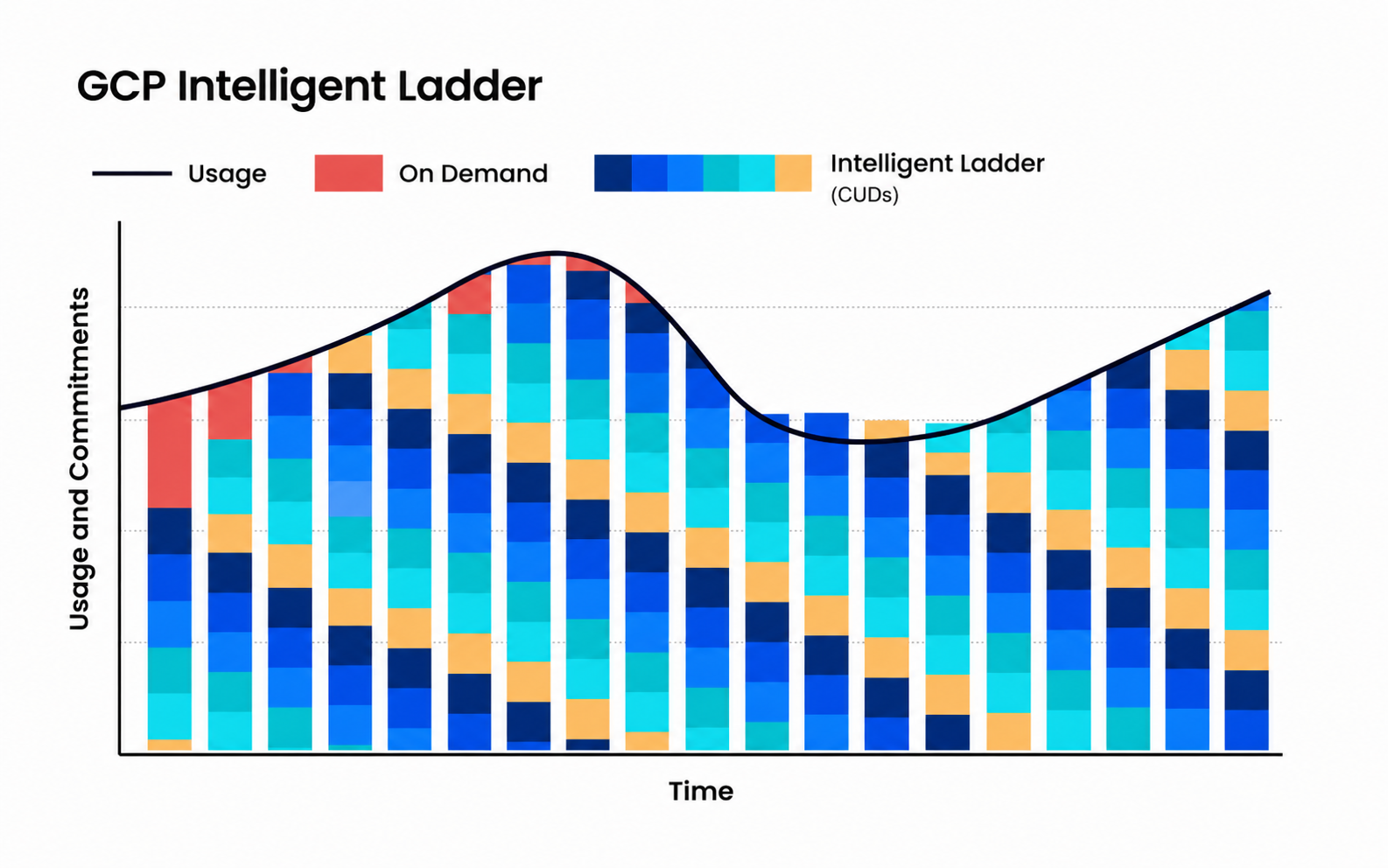
CUDs offer larger discounts (up to ~50% off, depending on the service), but they require you to commit ahead of time. They’re designed to lower the cost of your predictable baseline usage. The tradeoff is flexibility: if your footprint shrinks, shifts regions, or changes architecture, you can end up paying for commitment you don’t fully use.
This is where teams often look for a GCP committed use discount calculator or GCP savings plan calculator to determine how much baseline is safe to commit and how much risk they’re taking on if usage drops. nOps offers a free Savings Analysis to walk through your GCP commitment questions.
Once you know which rate model applies to Google Cloud Platform pricing, the next step is understanding what you’re being charged for on the compute side.
Compute costs in GCP come down to the resources you run (VMs, containers, serverless), how they’re sized, and how long they run.
For virtual machines, cost is driven primarily by:
A GCP VM cost calculator typically multiplies vCPU + memory rates by hours used, then adds disk and network charges. The biggest drivers are instance sizing and how consistently the VM runs — which is why rightsizing and uptime assumptions matter more than small price differences between machine families.
Cloud Functions (and other serverless compute like Cloud Run) are priced differently than VMs. Instead of paying for provisioned capacity, you pay for:
Costs scale directly with usage. This can be very cost-efficient for bursty or low-volume workloads, but traffic spikes can increase bills quickly if not modeled properly.
With GKE, you’re paying for the underlying compute resources that run your containers — typically Compute Engine nodes — plus any additional control plane or management fees (depending on configuration). Cost drivers include:
Because clusters often maintain buffer capacity, container environments frequently have hidden idle cost unless tightly optimized.
Data services introduce a different pricing model. BigQuery typically charges for:
Query-heavy workloads can become expensive if not optimized, especially when large datasets are scanned repeatedly.
Managed databases (Cloud SQL, AlloyDB, Spanner, etc.) combine:
Here, cost is often tied to provisioned capacity rather than pure usage, which makes baseline sizing decisions critical.
Start by writing down the inputs a calculator actually needs: what runs, how big it is, how long it runs, and how much it changes.
Capture your baseline vs peak (hours running and scaling), where it runs (regions/zones), and the big volume drivers (GB stored, GB transferred, requests/jobs/queries).
| If your workload is… | Usually model it as… | What to capture for estimation |
|---|---|---|
| Stable baseline services | Compute Engine VMs | vCPU/RAM size, hours running, autoscaling rules |
| Containerized apps | GKE | node sizing, node count range, cluster overhead, idle headroom |
| Event-driven / spiky | Cloud Functions / Cloud Run | requests, avg duration, memory per request, concurrency |
| Fault-tolerant batch | Spot VMs | average runtime, interruption tolerance, fallback capacity |
Storage estimates get messy because you’re rarely paying for “GB stored” alone. Real bills include class choices, replication, retrieval, and the cost of moving data back out.
Start by mapping data into buckets: what must be hot, what can be infrequent access, and what can be archival. Then layer in growth and access behavior. If the data is read often or moved across regions, those “secondary” costs can dominate the line item.
| Network cost you should model | What to measure | Why it matters |
|---|---|---|
| Internet egress | GB/month to users/partners | Often the biggest surprise |
| Inter-region transfer | GB/month between regions | Architecture decisions multiply costs |
| Load balancers | GB processed + LB type | Frequently overlooked line item |
| CDN | % cache hit + GB offloaded | Can reduce egress, but isn’t free |
Now take your raw totals (compute hours, requests, GB stored, GB transferred) and apply pricing levers in this order:
Google Cloud Storage pricing is primarily determined by storage class, which reflects how frequently data is accessed. Standard is designed for active data with the highest storage cost but no retrieval fees. Nearline, Coldline, and Archive progressively lower the per-GB storage price in exchange for higher retrieval costs and minimum storage durations. The tradeoff is simple: the less frequently you access data, the cheaper it is to store — but the more expensive it is to retrieve.
Storage bills often include more than capacity charges. In addition to GB stored, costs may include:
After compute and storage, network and data transfer is often the next major driver of GCP spend.
In Google Cloud, ingress (data entering GCP) is generally free, while egress (data leaving GCP) is charged — and the destination determines the rate. Egress to the public internet is typically the most expensive, while transfers within the same region may be free or lower cost depending on the service. Charges apply when data leaves a region, leaves a VPC, or exits to another cloud or on-prem environment.
For user-facing applications, APIs, media delivery, analytics exports, and backups sent off-platform, egress can quickly become one of the largest and most volatile components of monthly spend because it scales directly with traffic volume rather than provisioned capacity.
Inter-region traffic is billed when data moves between different Google Cloud regions, even if it stays within your own project. This commonly occurs when compute runs in one region while databases or storage reside in another, or when multi-region architectures replicate data for resilience. Pricing varies based on source and destination regions, and at scale, even internal service-to-service communication can generate substantial cost.
Architectures designed for redundancy, disaster recovery, or global performance often multiply inter-region transfer charges if data synchronization is frequent or continuous.
One of the most common forecasting mistakes is leaving outbound data transfer out of the estimate entirely. Egress doesn’t map cleanly to a single infrastructure line item, so teams focus on what they can easily size (compute, storage, databases) and treat network as incidental — but the result is a forecast that’s structurally understated from the start.
The fix is treating egress as a first-class input tied to real behavior: users, request volume, response size, exports, and integrations. Because outbound traffic scales with adoption and feature usage, small assumptions compound quickly.
If you’re using Google Cloud at any real scale, cost management quickly become a moving target. nOps takes all of the manual work and complexity out of GCP cost optimization by automatically maximizing your savings.
Instead of relying on infrequent, bulk CUD purchases, nOps uses intelligent commitment laddering—automatically committing in small, continual increments that align to your real usage. Coverage is recalculated and adjusted as demand changes, creating frequent expiration opportunities so commitments can flex up or down without sacrificing discounts. This approach extends savings beyond a static baseline, reduces long-term lock-in risk, and helps capture discounts across variable and spiky workloads with zero manual effort.
nOps only gets paid after it saves you money. There’s no upfront cost, no long-term commitment, and no risk or downside — if nOps doesn’t deliver measurable savings, you don’t pay.
In addition to visibility on your GCP cloud expenses, nOps gives you full visibility into your resources and spending across other cloud providers with forecasting, budgets, anomaly detection, and reporting to spot issues early and validate commitment savings. That visibility flows directly into automated cost allocation, so you can instantly allocate costs across project, environment, team, application, service, and region without any manual tagging or effort.
Want to see it in practice? to walk through CUD coverage, cost visibility, allocation, and anomaly protection in your Google Cloud Platform environment.
nOps manages $3B+ in cloud spend and was recently rated #1 in G2’s Cloud Cost Management category.
Let’s dive into a few FAQ about GCP pricing calculators and FinOps tools that can help estimate GCP costs.
Last Updated: June 7, 2026, Cost Optimization
Last Updated: June 7, 2026, Cost Optimization
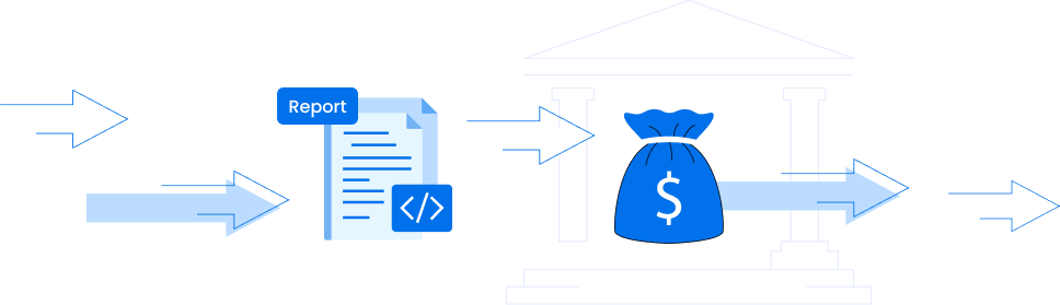
AI-powered rate optimization with risk-free guarantee