Simple Regularized Linear and Polynomial Regression

👁 Image by Author

Introduction

Linear and polynomial regression are extensively utilized in the field of data analytics for the purpose of future trend prediction in sectors like medicine, finance as well as engineering obviously. There is no perfect regression that exists but we can make it close to perfect by tuning parameters like degrees of the polynomials. For linear regression, we cannot increase the degree but we can make the best fitting based on the training data we have. However, the question is what might be the impact of this tuning on the test data. Will the model be as perfect as it is on the training data or there will more variance? What if we can introduce a bias in the model? That’s all we are going to discuss.

Linear Regression

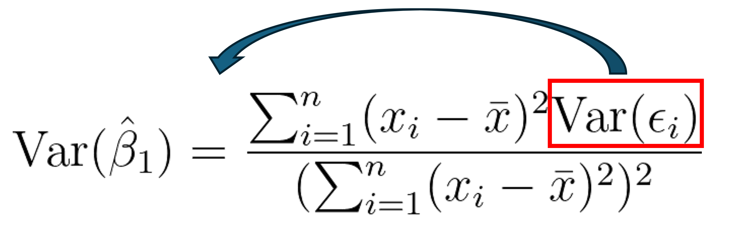
When performing linear regression, the best fitting line tends to minimize the squared error. The error can be positive or negative depending on which side the data point falls. Therefore, the squared term is taken to have the squared error and the fitting line is that line which corresponds to the least amount of error.

👁 Positive and negative error in regression [Image by Author]

The same thing happens when fitting the data with a polynomial. The least squared error line/curve can be interpreted by R-square value which essentially tells us how much variation can be described by the independent variables.

Typically in ML applications, we have training and test dataset where we fit the data using the training dataset and test it on the remaining data to find out how effective the model is. For this purpose, the whole dataset is usually divided into two sets: training and test dataset. We need to find the line/curve that best fits the training data. To achieve this, we may overfit the data and the model becomes highly experienced on the training data and in the end, it performs poorly on any test data or any data that it has not seen yet.

This is the essence of the bias-variance tradeoff phenomenon. When we have low bias in the model developed, there will be high variance in the test data when the model is deployed. By introducing bias, we can minimize the variance in the end.

Bias-variance tradeoff explained simple

Suppose we have the following training data which we fit with a linear model. The mean squared error for this dataset is 0.095 which is small.

👁 Training data with linear fit [Image by Author]

Also assume that the red dots are test dataset. It is clearly evident that when we extend the linear fit, there will last amount of error. In other words, there will be high variance. The mean squared error for this dataset is 8.41 which is higher compared to the residual squared error from training dataset.

👁 Training (blue) and test (red) data [Image by Author]

Let’s apply a bias to this model. Ridge regression introduces a bias to the model depending on the alpha value. The alpha value can be determined by ridge cross validation which automates the process of selecting the best alpha value. Alpha is therefore, a measure of introducing a penalty to the model. Higher the value of alpha, the more the model punishes the coefficients of the model. This is because it wants to reduce the impact of that independent variable on the dependent variable. If the alpha value is too high, it makes the linear fit a total flat line making the coefficient effectively 0 and remove the influence of the independent variable.

Let’s apply ridge regression on the same dataset with alpha = 0.1 to visualize the impact.

👁 Ridge regression with alpha = 0.1 [Image by Author]

As expected, the value of the coefficient has been reduced and we can see the effect of the penalty. The mean squared error for this dataset is 6.88 which is smaller compared to the residual square error from the model without the penalty. Therefore, by introducing a bias to the model, we have reduced the residual error on test data and also achieved lower variance. When we have high alpha value, the model turns into a flat line as below.

👁 Ridge regression with alpha = 100 [Image by Author]

Takeaway

1. Alpha value is a measure of penalty. It can be optimized using cross validation.
2. Higher alpha value results in smaller value of model coefficients. Thus it reduces the influence of the independent variable by introducing a bias.
3. Introducing a bias to model essentially reduces the variance in the test data.

Polynomial regression

The ridge regression can also applied to polynomial models. The same findings are true for polynomial regression. Let’s work on the "Fish" dataset under GPL 2.0 license. There are 5 independent variables and one response variable. When we increase the degree of the polynomial to find the best fit on the dataset, it increases the value of some coefficients which makes it more dominant than other independent variables. It is evident from the following figure (weight vs length data is used) where the x-axis represents the polynomial degree and y-axis represents the coefficient value. What does it mean actually? High coefficient value means we are putting more emphasize on a feature which makes it a very good predictor of the response variable while suppressing other features. This leads to overfitting on the training data which is not desired.

👁 High coefficient value from high degree of polynomial [Image by Author]

We can utilize Kernel Ridge for the purpose of penalizing the model coefficients. But let’s first fit the data with a polynomial of degree=5.

👁 Fish weight vs length data fitted by polynomial with degree = 5 [Image by Author]

The kernel ridge model with small value of alpha produces similar fitting curve.

👁 Fish weight vs length data fitted by polynomial with degree = 5 after application of kernel ridge with alpha = 0.5 [Image by Author]

When alpha in increased, the complexity of the model reduces. It is evident from the figure below where alpha = 5e15.

👁 Fish weight vs length data fitted by polynomial with degree = 5 after application of kernel ridge with alpha = 5e15 [Image by Author]

Takeaway

1. Scikit-learn’s kernel ridge is used for polynomial ridge regression.
2. Smaller alpha value mimics the same model with a regular polynomial fitting.
3. Higher alpha value reduces the model complexity.

Conclusion

Ridge regression (L2 regularization) is simply a way to reduce the impact of overfitting the model on training dataset. It can work on both linear as well as non-linear model to penalize the coefficients. Cross validation step is required to determine a best value of alpha which defines the level of penalizing the coefficients and therefore, make the model’s variance reduced when applied to test dataset. In brief, by introducing a small bias (depend on alpha level), we can regularize the model’s variance on test dataset to achieve enhanced performance.

Share This Article

• Share on Facebook
• Share on LinkedIn
• Share on X