Data Science

👁 Photo by Maximilian Weisbecker on Unsplash

In this article, I’ll walk through how to build models to predict the survival status of the Titanic passengers in Python. The methodology used here could also be applied to other similar use cases.

For added context, you can refer to the previous article, Exploratory Data Analysis & Visualization in Python, to read more about the Titanic data exploration and visualization in Python.

The titanic data can be downloaded from the Kaggle website.

---

1. Handling Missing Data

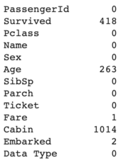
There are 4 predictors that contain missing data – Age, Fare, Cabin, and Embarked.

👁 Missing value count

Age

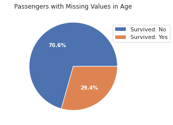
For the missing data in age, we can (1) refill the n/a values with mean or median, or (2) categorize the n/a values as a separate category. I chose the second option given that the n/a category could have useful information for predicting the survival status.

👁 Analyzed in the previous article

The missing data in age was categorized as a category. For the remaining non-missing values, one way to categorize them is by manually defining the number of age bins and the bin size.

👁 Survival rates by age bins

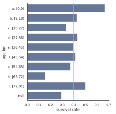
In the chart above, the non-missing age values were categorized into 9 age bins. It’s easy to change the age_bin_size input in the categorize_age function to test out a different number of age bins and see which one makes sense. This approach is a bit arbitrary. I prefer another way to select age bins – using the K-Means clustering method.

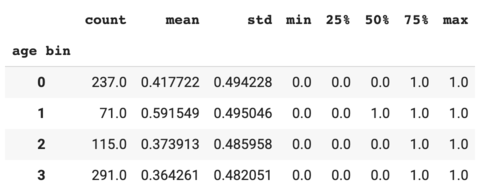
Apply K-Means clustering to the non-missing age data.

👁 Age range for each age bin defined by k-means

👁 Survival rates by age bin

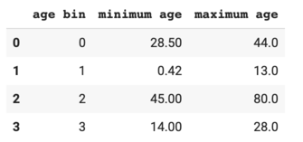
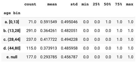
As shown in the output table, children (age bin #1 with age ranged from 0 to 13) had the highest survival rates compared to the other age groups.

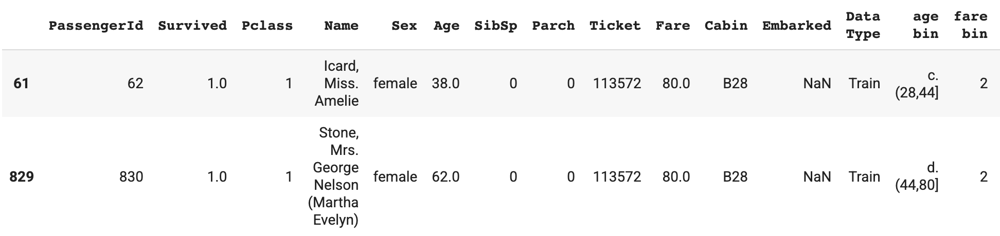
Based on the age bins and bin sizes above, I created a new variable called "age bin".

👁 Survival rates by age bins

Fare

Only one passenger didn’t have fare data.

👁 Passenger without fare data

This passenger had a third class ticket. I refilled the fare data by the average fare in the 3rd class tickets.

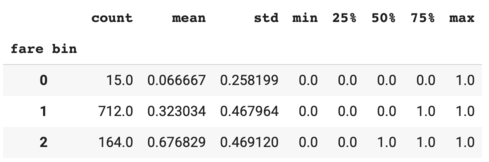
Next, create the fare bins using the K-Means clustering method. In the previous article, I found that passengers with complementary tickets had a very low survival rate. So I coded the $0 fare as a separate category.

👁 Survival rates by fare bins

Cabin

There are too many missing values in Cabin. I decided to drop this column.

Embarked

Two passengers didn’t have Embarked data, and they both had the first class tickets.

👁 Passengers without Embarked data

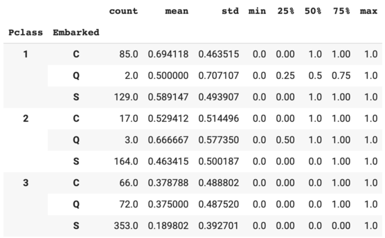
We can check the Embarked median by Pclass.

👁 Pclass by Embarked metrics

The median of Embarked in Pclass = 1 is S. Refill the missing Embarked data with S.

2. Engineering New Features

Travel group size

It’d be interesting to group people by the ticket number.

👁 Survival rate by travel size

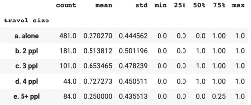
Note that the survival rate increased as the travel size increased except for the traveling group with 5+ people.

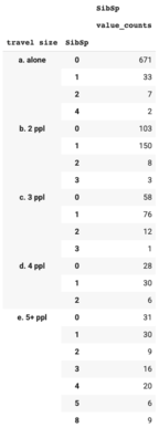
Next, use SibSp and Parch to double check if the travel size variable is defined correctly.

The number of people traveling together (travel group size) should be ≥ the number of siblings / spouses aboard (SibSp) + 1. Here we can see that this was not the case for a few passengers. This indicated that a few passengers traveled together as a family but they didn’t purchase the same ticket numbers.

👁 Image

Update the travel size based on SibSp.

I updated the travel size based on Parch using the same approach.

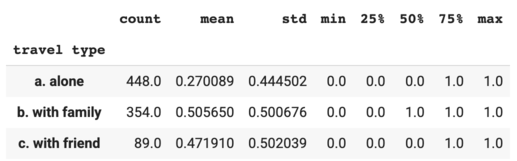
Travel group type

I created a new variable to specify if the passenger was traveling alone, with family or with friend.

👁 Survival rate by travel type

Title

There might be some information in the Name variable. I extracted the title from Name and created a new variable called "title".

👁 Passenger count by title

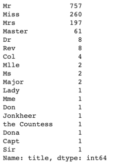
Group all the other titles except for the top 4 into an "other" category.

👁 Survival rate by title group

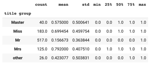
The title group variable is probably highly correlated with Sex and age bin.

3. One-Hot Encoding

One-hot encoding is used to convert categorical variables that contain label values (e.g. male, female) to numeric values (0 or 1).

First, let’s drop the columns that won’t be used in modeling. I dropped SibSp and Parch because they are probably be highly correlated with travel size.

👁 Example data in df_model

👁 Data types

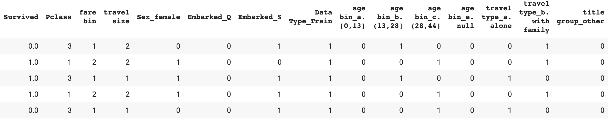
Next, apply the one-hot encoding to columns that have the object type.

I dropped some columns to prevent high correlations in the data. Using Sex as an example, keeping Sex_female only would be sufficient – if Sex_female = 0, then that indicates the gender is male.

👁 Example data in data_dummies

4. Correlation

I used Cramer’s V correlation given that the variables are either nominal or ordinal.

👁 Correlation heatmap

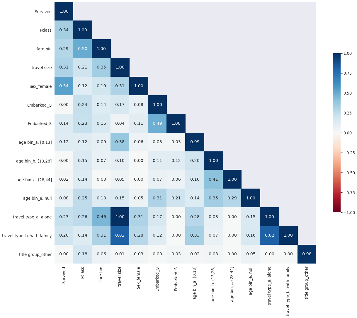
It’s not surprising to see that travel type and travel size variables are highly correlated. I decided to drop the travel type variables.

5. Modeling

Finally, the data is ready for modeling!

👁 Data shape for training and testing data

Fit the training data for a selected list of models. Use cross validation to calculate the accuracy scores.

👁 Model accuracy scores

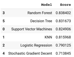
Random Forest gave the highest accuracy score – ~84%.

Visualize the feature coefficients using the Logistic Regression model to get a sense of how the model works.

👁 Feature coefficients in Logistic Regression model

👁 Feature coefficients to predict survival status

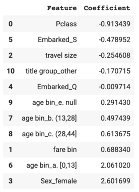
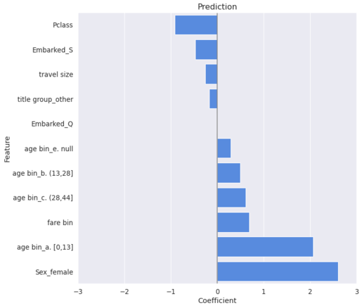
As to the feature coefficients, female passengers were much more likely to survive compared to the male passengers, and children were much more likely to survive compared to the other age groups. On the other hand, passengers with a lower ticket class were less likely to survive compared to the other passengers. This validated the hypotheses formed from the exploratory analysis.

Thanks for reading! Feel free to leave a comment and let me know what you think.

Share This Article

• Share on Facebook
• Share on LinkedIn
• Share on X