Introduction to Time series Modeling With -ARIMA

This article was published as a part of the Data Science Blogathon

Introduction

Often wondered if we could know what would the price of bitcoin be 6 months from now or how would your favourite stocks look like in a week, now you can predict all of these with time series modelling. One of the most commonly used data science applications is time series forecasting. As the name suggests, a time series forecast is predicting the future value of a variable by looking into the past history with the help of some additional features which are likely to affect those variables. The algorithms are designed in such a way that it looks at the trends of the past and forecasts the future values.

There are dozens of algorithms which can do time series forecast. There are the basic ones like Auto Regression, Moving average, ARMA, ARIMA, simple exponential smoothing, Holt Winter’s method, linear regression to advanced ones like the multiple linear regression, LSTM (Long Short Term Memory), Artificial neural networks and many more. Based on the data set and the supporting features we can make an informed decision and finalise the model.

Image Source: Google Images https://www.analyticssteps.com/blogs/introduction-time-series-analysis-time-series-forecasting-machine-learning-methods-models

Let us look into time series modelling using ARIMA.

What is ARIMA?

Autoregressive integrated moving average or popularly known as ARIMA is a very widely used time series forecasting technique. Before starting prediction with ARIMA let us understand the concept of stationary. A time-series prediction is done only if the dataset is stationary. A dataset is said to be stationary if its mean and variance remains constant over time. A stationary dataset does not have trend or seasonality.

When forecasting using time series models, we assume that each data point is independent of the other and this can be confirmed if the series is stationary. To check if a time series is stationary or not, just plot the observations against time and you can implement dicker-fuller’s test to check.

We can use the differencing technique to make the time series stationary, just subtract the previous observation for the next observation. This is 1^st degree differencing. If the series is still not stationary you can do the differencing again until the series becomes stationary. Generally, 1 or 2 degrees of difference is sufficient to make the series stationary.

Now that we know that the series is stationary, let look at the ARIMA model in detail. The ARIMA algorithm is made of the following components.

The AR stands for Auto Regression which is denoted as P, the value of P determines how the data is regressed on its past values.

The I stands for Integrated or the differencing component which is denoted as d, the value of d determines the degree of difference used to make the series stationary.

The MA stands for Moving Average which is denoted as q, the values of q determines the outcome of the model depends linearly on the past observations and the same goes for the errors in forecasting as they also vary linearly.

ARIMA model in Python

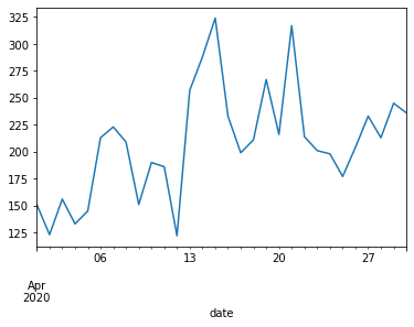
Now that we have an understanding of the ARIMA model, let us try to implement it with the mask sales dataset in April 2020 and predict the sales for the next few days.

import pandas as pd
import matplotlib.pyplot as plt
from statsmodels.tsa.arima.model import ARIMA
from sklearn.metrics import mean_squared_error
from math import sqrt
mask_sale = pd.read_excel('Book1.xlsx',header=0, parse_dates=[0], index_col=0, squeeze=True)
#result = seasonal_decompose(mask_sale['no_of_mask'],model ='multiplicative')
print(mask_sale.head())
mask_sale.plot()
plt.show()

Let’s divide the data into a training set and test set so that we can train the model on 70% of the data observations and test it on the remaining 30% of the data.

X = mask_sale.values


size = int(len(X) * 0.7)
train, test = X[0:size], X[size:len(X)]
history = [x for x in train]
predictions = list()
# walk-forward validation
for t in range(len(test)):
 model = ARIMA(history, order=(5,1,0))
 model_fit = model.fit()
 output = model_fit.forecast()
 yhat = output[0]
 predictions.append(yhat)
 obs = test[t]
 history.append(obs)
 print('predicted=%f, expected=%f' % (yhat, obs))
# evaluate forecasts
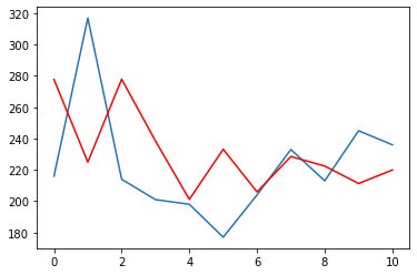
rmse = sqrt(mean_squared_error(test, predictions))
print('Test RMSE: %.3f' % rmse)
# plot forecasts against actual outcomes
plt.plot(test)
plt.plot(predictions, color='red')
plt.show()

Other times series models…

There are numerous time series models which can be used for forecasting time series data but the choice of the model totally depends on the problem statement. The ARIMA modelling technique which we looked at in this blog is the simple time series technique that makes the predictions without taking into consideration other factors which might be affecting our dependent variable.

The other advanced time series forecasting techniques like multiple linear regression has a dependent variable (our variable of interest) and many other dependent variables which influence the dependent variable. For example in house price dataset, the number of bedrooms or size od rooms, number of bathrooms, age of the house, etc are the independent variable or while predicting the weather, pressure, humidity, wind speed, temperature etc will be the independent variables which influence the sales of the houses. But never forget that not all independent variables will influence the dependent variables, so to make sure that the added independent variable is adding value to our model, just check the r squared and the adjusted r squared of these variables. If the adjusted r squared is less than the r squared then the variable is adding values to our model else we can ignore the other variables.

There are deep learning time series forecasting techniques like recurrent neural networks, long short term memory, gated recurrent unit etc which can overcome the shortcomings of the traditional forecasting techniques. The accuracy realised with these techniques is much higher compared to the traditional algorithms.

Footnote

It is always recommended to look at the data set and the problem statement before narrowing down on any time series modelling technique. Also, it’s better to explore more than just one model and then decide on the modelling techniques by looking at the accuracy of the prediction.

The media shown in this article are not owned by Analytics Vidhya and are used at the Author’s discretion.

Login to continue reading and enjoy expert-curated content.

Free Courses