Developing Vector AutoRegressive Model in Python!

This article was published as a part of the Data Science Blogathon

Introduction

A univariate time series is a series that contains only a single time-dependent variable whereas multivariate time series have more than one time-dependent variable. Each variable depends not only on its past values but also has some dependency on other variables.

Vector AutoRegressive (VAR)

Vector AutoRegressive (VAR) is a multivariate forecasting algorithm that is used when two or more time series influence each other.

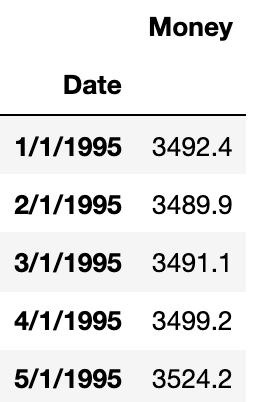
Let’s understand this be one example. In general univariate forecasting algorithms (AR, ARMA, ARIMA), we predict only one time-dependent variable. Here ‘Money’ is dependent on time.

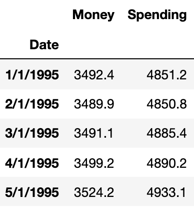
Now, suppose we have one more feature that depends on time and can also influence another time-dependent variable. Let’s add another feature ‘Spending’.

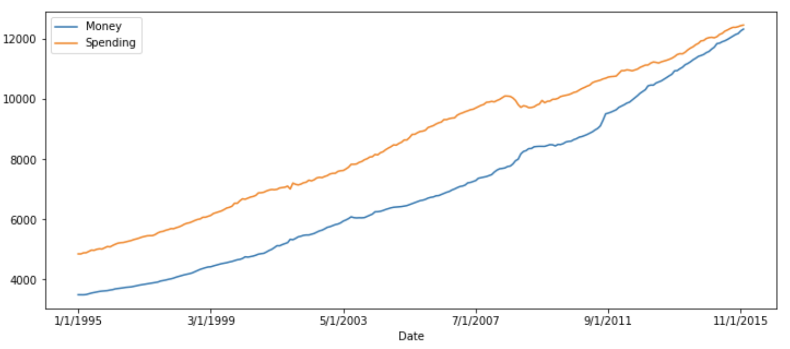
Here we will predict both ‘Money’ and ‘Spending’.  If we plot them, we can see both will be showing similar trends.

The main difference between other autoregressive models (AR, ARMA, and ARIMA) and the VAR model is that former models are unidirectional (predictors variable influence target variable not vice versa) but VAR is bidirectional.

A typical AR(P) model looks like this:

Here:
c-> intercept
$phi$ -> coefficient of lags of Y till order P
epsilon -> error

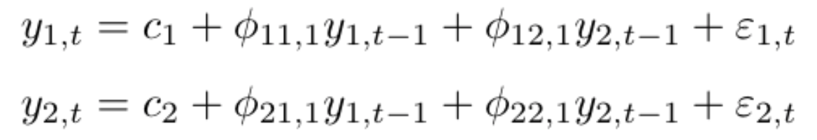
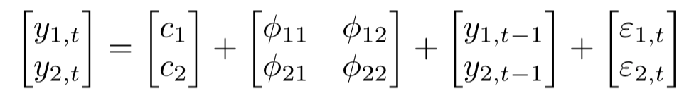
A K dimensional VAR model of order P, denoted as VAR(P), consider K=2, then the equation will be:

For the VAR model, we have multiple time series variables that influence each other and here, it is modelled as a system of equations with one equation per time series variable. Here k represents the count of time series variables.

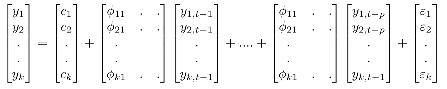
In matrix form:

The equation for VAR(P) is:

VAR Model in Python

Let us look at the VAR model using the Money and Spending dataset from Kaggle. We combine these datasets into a single dataset that shows that money and spending influence each other. Final combined dataset span from January 2013 to April 2017.

Steps that we need to follow to build the VAR model are:

1. Examine the Data
2. Test for stationarity
2.1 If the data is non-stationary, take the difference.
2.2 Repeat this process until you get the stationary data.
3. Train Test Split
4. Grid search for order P
5. Apply the VAR model with order P
6. Forecast on new data.
7. If necessary, invert the earlier transformation.

1. Examine the Data

First import all the required libraries

import pandas as pd
import numpy as np
import matplotlib.pyplot as plt
%matplotlib inline

Now read the dataset

money_df = pd.read_csv('M2SLMoneyStock.csv')
spending_df = pd.read_csv('PCEPersonalSpending.csv')
df = money_df.join(spending_df)

import pandas as pd
import numpy as np
#import matplotlib.pyplot as plt

money_df = pd.read_csv('M2SLMoneyStock.csv')
spending_df = pd.read_csv('PCEPersonalSpending.csv')
df_concat = pd.merge(money_df, spending_df, on='Date', how='outer')
df_concat=pd.DataFrame(df_concat)
print(df_concat.shape)
print(df_concat.head())

2. Check for Stationarity

Before applying the VAR model, all the time series variables in the data should be stationary. Stationarity is a statistical property in which time series show constant mean and variance over time.

One of the common methods to perform a stationarity check is the Augmented Dickey-Fuller test.

In the ADF test, there is a null hypothesis that the time series is considered non-stationary. So, if the p-value of the test is less than the significance level then it rejects the null hypothesis and considers that the time series is stationary.

def adf_test(series,title=''):
 """
 Pass in a time series and an optional title, returns an ADF report
 """
 print(f'Augmented Dickey-Fuller Test: {title}')
 result = adfuller(series.dropna(),autolag='AIC') # .dropna() handles differenced data
 labels = ['ADF test statistic','p-value','# lags used','# observations']
 out = pd.Series(result[0:4],index=labels)
 for key,val in result[4].items():
 out[f'critical value ({key})']=val
 print(out.to_string()) # .to_string() removes the line "dtype: float64"
 if result[1] <= 0.05:
 print("Strong evidence against the null hypothesis")
 print("Reject the null hypothesis")
 print("Data has no unit root and is stationary")
 else:
 print("Weak evidence against the null hypothesis")
 print("Fail to reject the null hypothesis")
 print("Data has a unit root and is non-stationary")

Check both the features whether they are stationary or not.

adf_test(df['Money'])

Augmented Dickey-Fuller Test: 
ADF test statistic 4.239022
p-value 1.000000
# lags used 4.000000
# observations 247.000000
critical value (1%) -3.457105
critical value (5%) -2.873314
critical value (10%) -2.573044
Weak evidence against the null hypothesis
Fail to reject the null hypothesis
Data has a unit root and is non-stationary

Now check the variable ‘Spending’.

adf_test(df['Spending'])

Augmented Dickey-Fuller Test: 
ADF test statistic 0.149796
p-value 0.969301
# lags used 3.000000
# observations 248.000000
critical value (1%) -3.456996
critical value (5%) -2.873266
critical value (10%) -2.573019
Weak evidence against the null hypothesis
Fail to reject the null hypothesis
Data has a unit root and is non-stationary

Neither variable is stationary, so we’ll take a first-order difference of the entire DataFrame and re-run the augmented Dickey-Fuller test.

df_difference = df.diff()

adf_test(df_difference['Money'])

Augmented Dickey-Fuller Test: 
ADF test statistic -7.077471e+00
p-value 4.760675e-10
# lags used 1.400000e+01
# observations 2.350000e+02
critical value (1%) -3.458487e+00
critical value (5%) -2.873919e+00
critical value (10%) -2.573367e+00
Strong evidence against the null hypothesis
Reject the null hypothesis
Data has no unit root and is stationary

adf_test(df_difference['Spending'])

Augmented Dickey-Fuller Test: 
ADF test statistic -8.760145e+00
p-value 2.687900e-14
# lags used 8.000000e+00
# observations 2.410000e+02
critical value (1%) -3.457779e+00
critical value (5%) -2.873609e+00
critical value (10%) -2.573202e+00
Strong evidence against the null hypothesis
Reject the null hypothesis
Data has no unit root and is stationary

3. Train-Test Split

We will be using the last 1 year of data as a test set (last 12 months).

test_obs = 12
train = df_difference[:-test_obs]
test = df_difference[-test_obs:]

4. Grid Search for Order P

for i in [1,2,3,4,5,6,7,8,9,10]:
 model = VAR(train)
 results = model.fit(i)
 print('Order =', i)
 print('AIC: ', results.aic)
 print('BIC: ', results.bic)
 print()

Order = 1
AIC: 14.178610495220896

Order = 2
AIC: 13.955189367163705

Order = 3
AIC: 13.849518291541038

Order = 4
AIC: 13.827950574458281

Order = 5
AIC: 13.78730034460964

Order = 6
AIC: 13.799076756885809

Order = 7
AIC: 13.797638727913972

Order = 8
AIC: 13.747200843672085

Order = 9
AIC: 13.768071682657098

Order = 10
AIC: 13.806012266239211

VAR(5) returns the lowest score and after that again AIC starts increasing, hence we will build the VAR model of order 5.

5. Fit VAR(5) Model

result = model.fit(5)
result.summary()

 Summary of Regression Results 
==================================
Model: VAR
Method: OLS
Date: Thu, 29, Jul, 2021
Time: 15:21:45
--------------------------------------------------------------------
No. of Equations: 2.00000 BIC: 14.1131
Nobs: 233.000 HQIC: 13.9187
Log likelihood: -2245.45 FPE: 972321.
AIC: 13.7873 Det(Omega_mle): 886628.
--------------------------------------------------------------------
Results for equation Money
==============================================================================
 coefficient std. error t-stat prob
------------------------------------------------------------------------------
const 0.516683 1.782238 0.290 0.772
L1.Money -0.646232 0.068177 -9.479 0.000
L1.Spending -0.107411 0.051388 -2.090 0.037
L2.Money -0.497482 0.077749 -6.399 0.000
L2.Spending -0.192202 0.068613 -2.801 0.005
L3.Money -0.234442 0.081004 -2.894 0.004
L3.Spending -0.178099 0.074288 -2.397 0.017
L4.Money -0.295531 0.075294 -3.925 0.000
L4.Spending -0.035564 0.069664 -0.511 0.610
L5.Money -0.162399 0.066700 -2.435 0.015
L5.Spending -0.058449 0.051357 -1.138 0.255
==============================================================================

6 Predict Test Data

The VAR .forecast() function requires that we pass in a lag order number of previous observations.

lagged_Values = train.values[-8:]

pred = result.forecast(y=lagged_Values, steps=12) 

idx = pd.date_range('2015-01-01', periods=12, freq='MS')
df_forecast=pd.DataFrame(data=pred, index=idx, columns=['money_2d', 'spending_2d'])

7. Invert the transformation

df_forecast['Money1d'] = (df['Money'].iloc[-test_obs-1]-df['Money'].iloc[-test_obs-2]) + df_forecast['money2d'].cumsum()
df_forecast['MoneyForecast'] = df['Money'].iloc[-test_obs-1] + df_forecast['Money1d'].cumsum()

df_forecast['Spending1d'] = (df['Spending'].iloc[-test_obs-1]-df['Spending'].iloc[-test_obs-2]) + df_forecast['Spending2d'].cumsum()
df_forecast['SpendingForecast'] = df['Spending'].iloc[-test_obs-1] + df_forecast['Spending1d'].cumsum()

Plot the Result

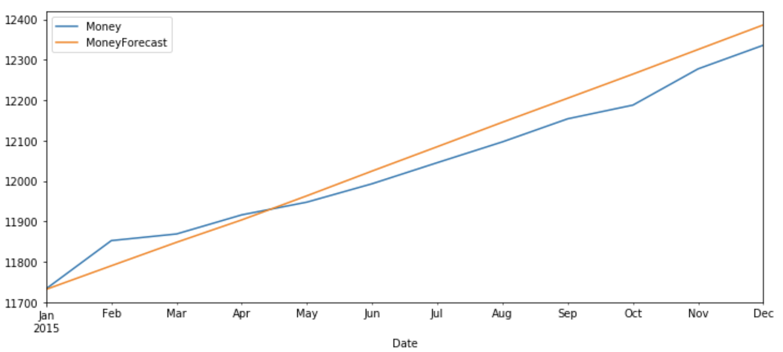
Now let’s plot the predicted v/s original values of ‘Money’ and ‘Spending’ for test data.

test_original = df[-test_obs:]
test_original.index = pd.to_datetime(test_original.index)

test_original['Money'].plot(figsize=(12,5),legend=True)
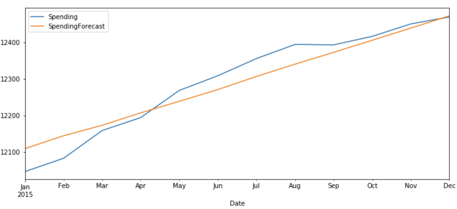
df_forecast['MoneyForecast'].plot(legend=True)

test_original['Spending'].plot(figsize=(12,5),legend=True)
df_forecast['SpendingForecast'].plot(legend=True)

The original value and predicted values show a similar pattern for both ‘Money’ and ‘Spending’.

Conclusion

In this article, first, we gave a basic understanding of univariate and multivariate analysis followed by intuition behind the VAR model and steps required to implement the VAR model in Python.

I hope you enjoyed reading this article. Please, let me know in the comments if you have any queries/suggestions.

Login to continue reading and enjoy expert-curated content.

Free Courses