Multiple Time Series Model Using Apache Spark and Facebook Prophet

This article was published as a part of the Data Science Blogathon.

Introduction

Let’s say you are a large retailer like Walmart, D-Mart, and you may deal with thousands and thousands of products and each product will have a different sale cycle. For example, woollen clothes will have more sales in winter, and swimming gears more in the summer season so If we have to predict or forecast the sales of every product then you end up doing separate time-series of each product present within these retailers.

One of the key challenges in this process is how do we create a model that can take the data and build thousand of time series models that we can test, evaluate and deploy. In this article, we will focus on how you can distribute your data and build multiple machine learning models (using Apache Spark and Facebook Prophet). Evaluation and deployment is still a tedious task that you have to do but here we will focus on how we can use Apache spark and Facebook Prophet to build a separate model for each product in a store.

What is Multiple Time Series Forecasting?

Multiple Time series forecasting similar time series to predict the same target using multiple models for corresponding shop or product. People majorly referred to it as Hierarchical forecasting because it deals with similar time series. Sales data, product data, tourist data for one city of different people from different places represent multiple time series modelling. People are sometimes confused between multiple time series and multivariate time series so let me tell you that both are completely different terms. Multivariate time series have more than one time-dependent variable but a single model is made While in Multiple time series different models is made concerning target and time-dependent variable. Further in this article, we will elaborate it in more detail with Hands-on practice. So let’s get started and set your Jupyter environment.

Brief on Dataset

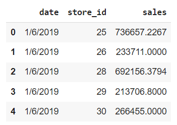
We are using Weekly sales Data. you can find the dataset here. We have the Date and weekly sales per store ID. So the date is by week. We have multiple stores and we have near about 50 weeks of data of 10 stores.

Hands-On Multiple Time Series Modeling

Loading Libraries

The first step is to install the required libraries. If you are working on google colab or a local Jupyter notebook then we need to install Apache Spark and Facebook Prophet.

!pip install pyspark
!pip install fbprophet
!pip install pyarrow = 0.15.1

• Pyspark is like Python binding for Spark. spark is written in scala so Pyspark provides a python binding to work with spark through python scripting.
• We are also installing pyarrow which is a package to efficiently transfer data across multiple tools and technologies So using it we can easily transfer the data between Python Pandas and Spark in a more efficient way rather than the traditional way of Pickling and Unpickling it.
• After that, we are installing Facebook Prophet which is used to model the time-series data.

After successful installation let’s load the required modules and libraries. we load visualization, data manipulation, and modelling libraries.

import pandas as pd
import matplotlib as mpl
import matplotlib.pyplot as plt
from fbprophet import Prophet
mpl.rcParams['figure.figsize'] = (10, 8)
mpl.rcParams['axes.grid'] = False

we are telling like to run a spark session in a local mode and assign it to an object. when we run this in a cluster mode then we can distribute the thousands of products across hundreds of nodes for fast query execution. we need to repartition the data based on a particular identifier which in our case is store id or Product ID.

from pyspark.sql import SparkSession
import pyspark
spark = SparkSession.builder.master('local').getOrCreate()

df = pd.read_csv("weekly_sales_data.csv")
df.shape

Basic Preprocessing

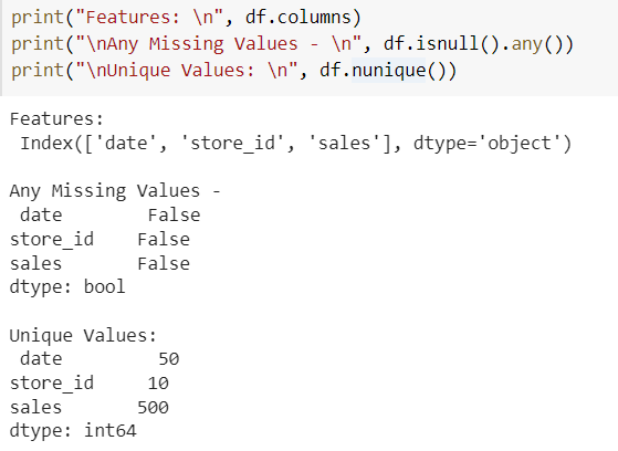
The first is to convert the date column from string type to Date type. After that let us check that is there any missing values and how many unique values we have in each column? Basically when we are running a Multiple time series then we are going to treat each store ID as separate time series so we are going to build 10 different models over here.

df['date'] = pd.to_datetime(df['date'], infer_datetime_format=True)

Visualize the Time-series data

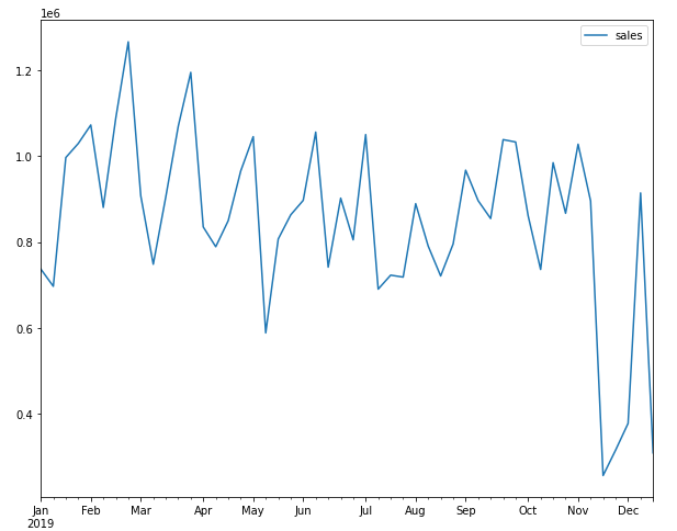
Now to visualize the time-series data of each store we are setting the date as an index and plot the graph for a particular store.

item_df = df.set_index('date')
item_df.query('store_id == 25')[['sales']].plot()
plt.show()

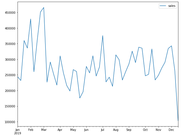
item_df.query('store_id == 41')[['sales']].plot()
plt.show()

We can see that there are lots of ups and downs. The pattern looks somewhat the same but the time series is different for a different store so we cannot build a single model over here to predict store sales because each store has a different increase and decrease graph.

Analyze the Dataset with Spark

Spark DataFrame

We have Pandas Dataframe and we have analyzed it. Now we will create a spark component so we will create a Spark DataFrame. you can also print schema of it to see the data type of columns. count function is used to count the rows in the dataset.

sdf = spark.createDataFrame(df)
sdf.printSchema() #data type of each col
sdf.show(5) #It gives you head of pandas DataFrame
sdf.count() #500 records

Spark is a lazy evaluation framework means until we apply any action it will not print anything only it prepares the DAG(Directed Acyclic Graph) which is a rough plan of execution. So we use an action statement to see the output like the show, count, etc.

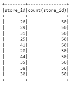
sdf.select(['store_id']).groupby('store_id').agg({'store_id': 'count'}).show()

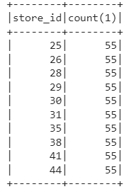
Now we will create a Temporary view to run the SQL queries on the dataframe. After this, we run a SQL query to find the count of each store ID and print it according to store ID. It will display the same table as shown in the above figure.

sdf.createOrReplaceTempView("sales")
spark.sql("select store_id, count(*) from sales group by store_id order by store_id").show()

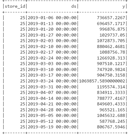
Spark is a distributed framework so what happens is multiple executors are running to read a chunk of data. we need to manually tell that our chunk of data is store ID so that all the data related to store are in one partition and when a model is built it uses all the store IDs together. If we don’t do this then different store IDs will be in different partitions. So we have to do it manually so we are running a below SQL statement in which we take a sum of sales(It will not do anything because we have data at the week level). The prophet expects the date as ds and the target column as Y.

sql = "SELECT store_id, date as ds, sum(sales) as y FROM sales GROUP BY store_id, ds ORDER BY store_id, ds"
spark.sql(sql).show()

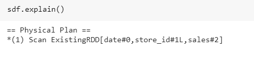
Whatever we have done till now in Spak context let us print the plan which is DAG prepared by a spark. So we observe that it is a single RDD function.

Repartition the Data

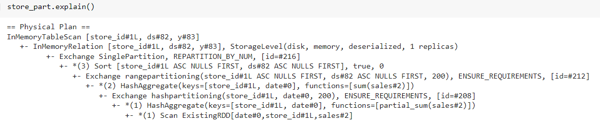
Now all the data is in a single partition but now I want it to break into Multiple partitions and for that, we will call the SQL statement on its top and repartition the data based on the Store ID column. And we will cache it so that we do not require to fetch data again and again. Machine Learning is an iterative process so we did not want to take data again and again.

Earlier we saw explain function only give an RDD function but now if we see it has done a lot of hash partitioning. Now we create a UDF function that will have facebook Prophet code. For that, we are importing Pyspark SQL data types to create a schema for our return object.

from pyspark.sql.types import *
result_schema = StructType([
 StructField('ds', TimestampType()),
 StructField('store_id', IntegerType()),
 StructField('y', DoubleType()),
 StructField('yhat', DoubleType()),
 StructField('yhat_upper', DoubleType()),
 StructField('yhat_lower', DoubleType())
])

So we create a result schema which states that the Timestamp is returned schema, Y is a value we are passing, That is the Prophet predicted value, That upper and lower are respective Upper and lower confidence intervals. So when Facebook Prophet predicts the value we can set the confidence Interval. Now from the Pyspark SQL function we will import Pandas UDF and UDF type and define a function that is the same as Python’s typical function.

from pyspark.sql.functions import pandas_udf, PandasUDFType
@pandas_udf(result_schema, PandasUDFType.GROUPED_MAP)
def forecast_sales(store_pd):
 model = Prophet(interval_width=0.95, seasonality_mode= 'multiplicative', weekly_seasonality=True, yearly_seasonality=True)
 model.fit(store_pd)
 future_pd = model.make_future_dataframe(periods=5, freq='w')
 forecast_pd = model.predict(future_pd)
 f_pd = forecast_pd[['ds', 'yhat', 'yhat_upper', 'yhat_lower']].set_index('ds')
 st_pd = store_pd[['ds', 'store_id', 'y']].set_index('ds')
 result_pd = f_pd.join(st_pd, how='left')
 result_pd.reset_index(level=0, inplace=True)
 result_pd['store_id'] = store_pd['store_id'].iloc[0]
 return result_pd[['ds', 'store_id', 'y', 'yhat', 'yhat_upper', 'yhat_lower']]

Here I am telling you that it is a grouped Map which means that when we create a Spark UDF then it operates row by row so for each row spark rates are going to execute it but the grouped map allows to be vectorized in a particular set of rows into the pandas UDF. In our case vectorization is based on Store ID so we are going to take a huge chunk of store ID and pass it as a vectorized object and run the Facebook Prophet and display the result.

from pyspark.sql.functions import current_date
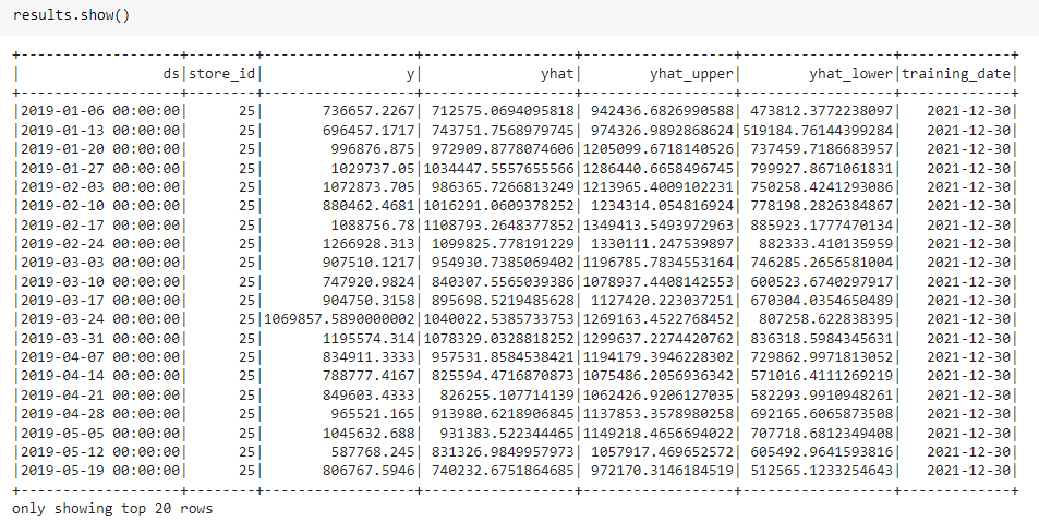
results = (store_part.groupby('store_id').apply(forecast_sales).withColumn('training_date', current_date()))
results.cache()
results.show()

~ The passage of data between spark and pandas dataframe is tedious and pyarrow makes it easy. Now we create a model object and initialize the Prophet object and define the confidence interval as 95 %. The Seasonality of the model is multiplicative and the reason we give it multiplicative is if we see the chart on top then there is no trend and there are lots of ups and downs so we give it as multiplicative because e have only one year of data so the product sales follow the same pattern. then we fit the data and create a future dataframe that stores the prediction for the next five periods and do prediction as per week. Then we pass future dataFrame so it creates the next 5 periods to predict. After all, is completed we prepare the data.

After this, we have pandas UDF function and pass the dataframe to it so we take the Pyspark function to show when we ran it to create some log. we cache the results and display the results. Now you can see for each store ID we have Y value, forecasted value, and upper and lower confidence interval, and the date I ran it. If you want to see the explanation of what we have done so we can print the explanation.

Coalesce the Partitions

Coalesce is the opposite of repartitioning so we take it and create one huge file which we can easily query. when I have multiple partitions then the data has to come from all partitions to analyze it so I am just unpartitioning it.

results.coalesce(1)
print(results.count())
results.createOrReplaceTempView('forecasted')
spark.sql("SELECT store_id, count(*) FROM forecasted GROUP BY store_id").show()

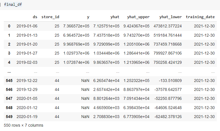
We have 10 Stores and we have predicted for 5 weeks for each store so we have a total of 550 records in a DataFrame. let us create a view of results to run  SQL queries on it. We convert this to Pandas Dataframe to visualize it better.

final_df = results.toPandas()

Visualize the Forecasted Sales 

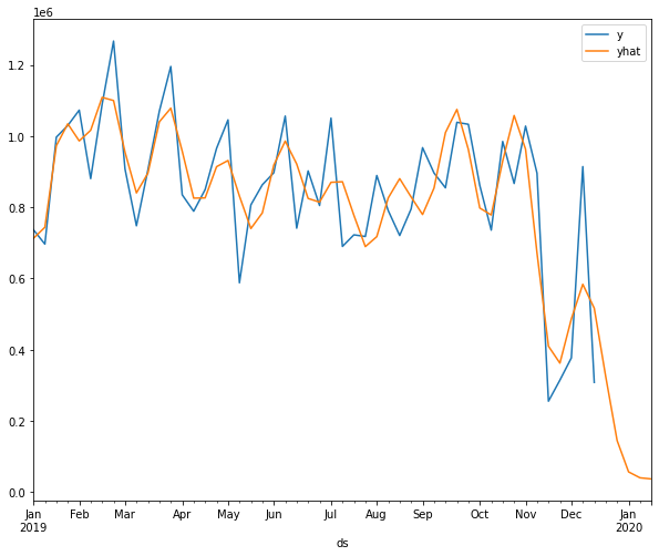
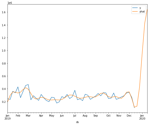
Visualize the results of a particular store concerning the correct labels and predicted labels. After observing the below graphs we can say that it has caught the pattern very well.

final_df = final_df.set_index('ds')
final_df.query('store_id == 25')[['y', 'yhat']].plot()
plt.show()

final_df.query('store_id == 41')[['y', 'yhat']].plot()
plt.show()

Conclusion

Apache Spark and Facebook Prophet are very handy functions to distribute your data seamlessly when you have a lot of products. you can run your models very fast, if you are running in your standalone Pandas or some other functions then we need to enable multi-processing but with spark, you are using multi-node capacity and run our hypothesis very fast. In this article, we have learned how to perform Multiple Time-series using Apache Spark and Facebook Prophet in any sales or product details dataset because every time series is different.

If you have any doubts or feedback, feel free to share them in the comments section below.

Connect with me on Linkedin.

Check out my other articles here and on Blogspot.

Thanks for giving your time!

Login to continue reading and enjoy expert-curated content.

Free Courses