 |
VOOZH | about |
|
VOOZH | about |
Conditional Formatting in Excel is more than just a feature—it’s a powerful tool transforming how you interact with data. Whether you’re managing a simple budget or analyzing complex datasets, Conditional Formatting helps you highlight important trends, patterns, and outliers with just a few clicks. In this article, we’ll explore how you can utilize this feature to make your data more visually appealing and informative.
At its core, Conditional Formatting allows you to apply specific formatting—such as colors, icons, or data bars—to cells based on the values they contain. This automatic formatting is triggered by rules you define, making it easy to spot critical data points or trends without manually sifting through numbers.
Also read: Microsoft Excel for Data Analysis
One of the simplest yet most effective uses of Conditional Formatting is highlighting cells based on their value. For instance, if you want to quickly identify which sales figures exceed a certain threshold, conditional formatting can help you. Here’s how:
Here’s how you can highlight cells based on values:
Choose the cells you want to format.👁 conditional formatting
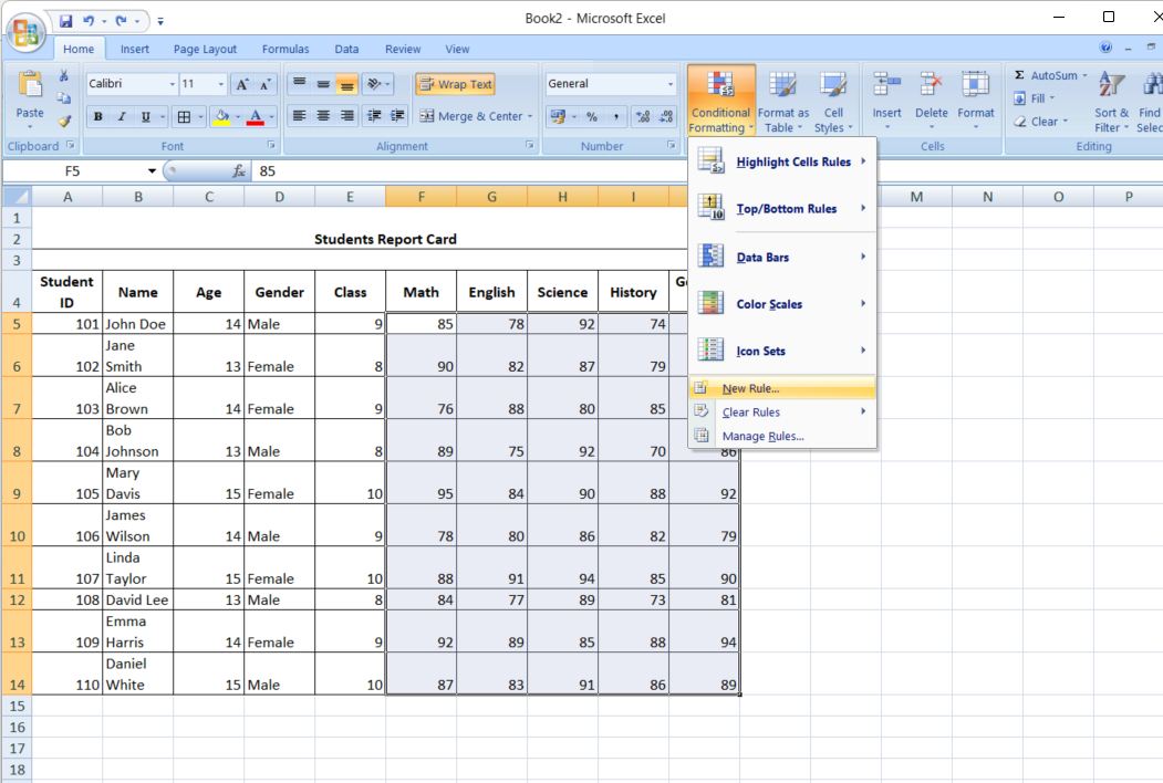
Find the Conditional Formatting option on the Home tab under the Styles group.👁 Conditional Formatting
Select “Highlight Cells Rules” and then “Greater Than.” Then, Enter the threshold value and choose your desired formatting style.👁 Conditional formatting
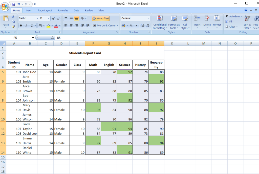
Click OK, and Excel will highlight the cells that meet your criteria.👁 conditional formatting
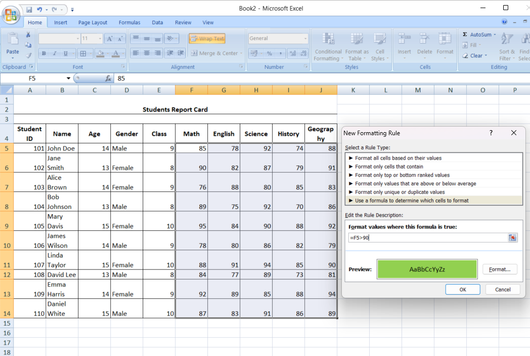
Excel’s flexibility shines when you use formulas to apply Conditional Formatting. This allows for more nuanced and customized rules. For example, you might want to highlight cells based on a condition that isn’t simply a comparison to a static value, like flagging sales higher than the previous month’s average.
Also read: A Comprehensive Guide on Advanced Microsoft Excel for Data Analysis.
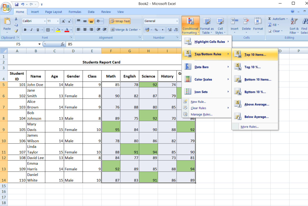
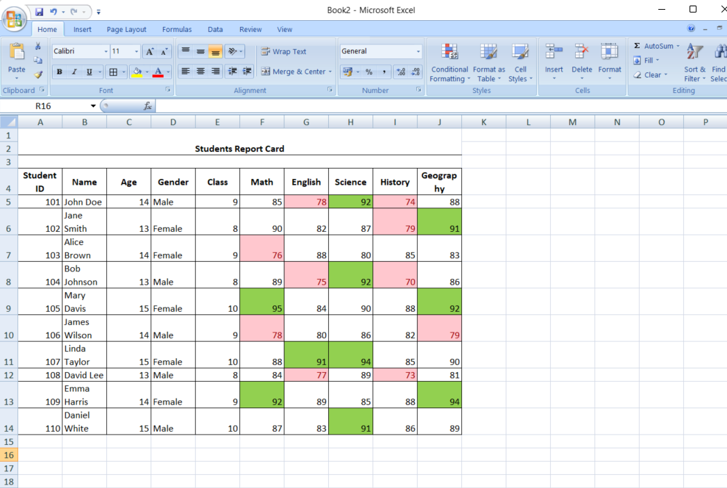
Conditional Formatting can also help you focus on the highest and lowest values in a dataset, such as identifying the top 10 performers or the bottom 5 sales figures.
Similarly, identifying duplicate entries is crucial in large datasets. Conditional Formatting can quickly highlight duplicates, helping you maintain data accuracy.
Here are the tips:
Conditional Formatting in Excel is not just a handy feature—it’s a game-changer for anyone who works with data. By leveraging this tool, you can turn a simple spreadsheet into a dynamic, visually appealing report highlighting key insights and trends at a glance. Whether you’re a data novice or an experienced analyst, mastering Conditional Formatting will enhance your ability to communicate data-driven stories effectively. So, the next time you’re in Excel, don’t just look at the numbers—let Conditional Formatting help you see the bigger picture.
Ans. Conditional Formatting in Excel lets you apply specific formatting to cells based on their values, such as highlighting, color scales, or icon sets.
Ans. Select the cells, go to the “Home” tab, click “Conditional Formatting,” choose a rule, and configure it as needed.
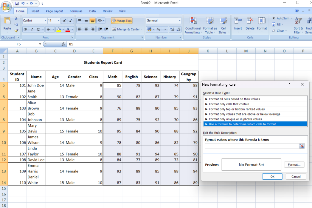
Ans. Yes, you can use formulas to create custom Conditional Formatting rules by selecting “Use a formula to determine which cells to format.”
Ans. Select the cells, go to “Conditional Formatting” in the “Home” tab, and choose “Clear Rules” to remove the formatting.
Hi, I am Pankaj Singh Negi - Senior Content Editor | Passionate about storytelling and crafting compelling narratives that transform ideas into impactful content. I love reading about technology revolutionizing our lifestyle.
GPT-4 vs. Llama 3.1 – Which Model is Better?
Llama-3.1-Storm-8B: The 8B LLM Powerhouse Surpa...
A Comprehensive Guide to Building Agentic RAG S...
Top 10 Machine Learning Algorithms in 2026
45 Questions to Test a Data Scientist on Basics...
90+ Python Interview Questions and Answers (202...
8 Easy Ways to Access ChatGPT for Free
Prompt Engineering: Definition, Examples, Tips ...
What is LangChain?
What is Retrieval-Augmented Generation (RAG)?
Edit
Resend OTP
Resend OTP in 45s