Linear Convolution using C and MATLAB

A key concept often introduced to those pursuing electronics engineering is Linear Convolution. This is a crucial component of Digital Signal Processing and Signals and Systems. Keeping general interest and academic implications in mind, this article introduces the concept and its applications and implements it using C and MATLAB.

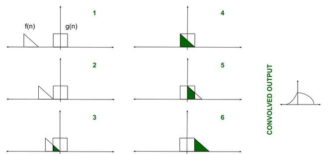
Convolution: When speaking purely mathematically, convolution is the process by which one may compute the overlap of two graphs. In fact, convolution is also interpreted as the area shared by the two graphs over time. Metaphorically, it is a blend between the two functions as one passes over the other. So, given two functions F(n) and G(n), the convolution of the two is expressed and given by the following mathematical expression:

or

👁 Linear convolution

So, clearly intuitive as it looks, we must account for TIME. Convolution involves functions that blend over time. This is introduced in the expression using the time shift i.e., g(t-u) is g(t) shifted to the right 'u' times). Additionally, how we characterize this time is also important. Before proceeding further, let us compile the prerequisites involved:

• Functions: Mathematically, we look at functions or graphs. However, it is important to note that the practical equivalent here is a Signal. We deal with the convolution of 2 signals.
• LTI Systems: Linear Time-Invariant Systems are systems or processes which produce a Linear and a Time-Invariant output i.e., the output satisfies Linearity (superposition rule) and does not change with time. Convolution is the relation between the input and output of an LTI system.
• Impulse Response: An impulse response is what you usually get if the system in consideration is subjected to a short-duration time-domain signal. Different LTI systems have different impulse responses.
• Time System: We may use Continuous-Time signals or Discrete-Time signals. It is assumed the difference is known and understood to readers. Convolution may be defined for CT and DT signals.

Linear Convolution: Linear Convolution is a means by which one may relate the output and input of an LTI system given the system's impulse response. Clearly, it is required to convolve the input signal with the impulse response of the system. Using the expression earlier, the following equation can be formed-

The reason why the expression is summed an infinite number of times is just to ensure that the probability of the two functions overlapping is 1. The impulse response is time-shifted endlessly so that during some duration of time, the two functions will certainly overlap. It may seem it would be careless on behalf of the programmer to run an infinite loop - the code may continue to execute for as long as the two functions do not overlap.

The solution lies in the fact LTI systems are being used. Since the functions do not change their values/shape over time (time-invariant), they can simply be slid closer to each other. Remember only the output is required, and it is not important 'when' the output is received. All manual calculations also depend on the same idea.

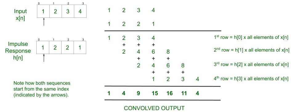
Explanation: Here's one technique that may be used while calculating the output:

• Take the input signal and impulse response as two separate single-row matrices.
• The first element of the impulse response is multiplied with every element of the input signal. This result is stored.
• The second element of the impulse response is multiplied with every element of the input signal. The result is shifted by one step to the right and stored.
• The above two steps are done for the remaining elements in the impulse response.
• Once all elements have been multiplied, align all the results under one another. Refer to the figure below.
• Vertically, add all the elements in each column.
• The resulting single row matrix is the convolved output.

👁 Explanation of Linear Convolution

Approach:

• Obtain the input signal and the impulse response as two distinct arrays.
• Obtain a time index sequence. The Time Index Sequence is a way by which MATLAB is informed about when our functions start. It starts at 0 by default i.e., [0 1 2 3 ........]. The 2nd sequence or the impulse response, however, needn't begin at the same time. One can choose to delay it or start it earlier. If it is introduced earlier by a second, then its Time Index Sequence should be input as [ -1 0 1 2 .......].
• Use user-defined functions. The function findconv() defines how the length of the output is calculated. Define 'ny' as the length of our x-axis in output. It is earlier defined as an array starting from 'nybegin' and extending till 'nyend'. The function calconv() is referenced in findconv() and calculates the actual output sequentially by taking different values of k and n, using 2 distinct for loops.
• For each value of n, the sum of outputs is calculated by taking a different X(k) value in each iteration.
• This result is stored in an array - y(n).
• Plot the result. The function stem() is used while plotting due to the fact that the input is DISCRETE in nature. If a continuous-time output were to be plotted, it wouldn't make any sense to use stem() as it would make it appear that the output is sampled. It is recommended to use plot(x_axis, y_axis) when plotting continuous values.
• Note: DO NOT vary the lengths of the time index sequence and the 1st and 2nd sequences. The stem() returns an error indicating that it is not able to establish the length of the x-axis in the output.

Below is the Matlab program to implement the above approach:

Input (any arbitrary set of numbers):

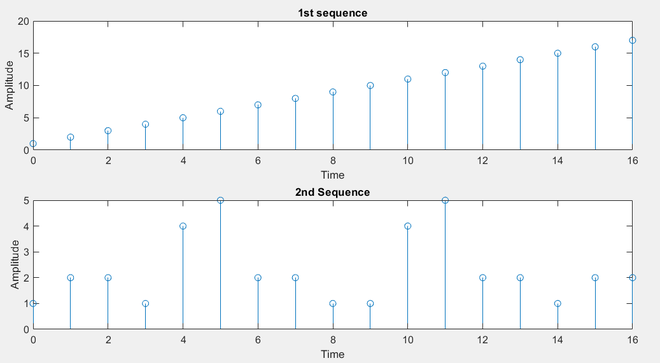
>> Enter the 1st Sequence: [1 2 3 4 5 6 7 8 9 10 11 12 13 14 15 16 17]
>> Enter the Time Index sequence: [0 1 2 3 4 5 6 7 8 9 10 11 12 13 14 15 16]
>> Enter the second sequence: [1 2 2 1 4 5 2 2 1 1 4 5 2 2 1 2 2]
>> Enter the Time Index sequence: [0 1 2 3 4 5 6 7 8 9 10 11 12 13 14 15 16]

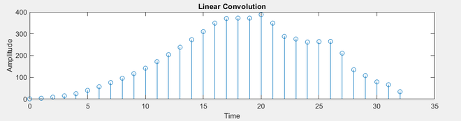
Output:

>> Columns 1 through 17
 1 4 9 15 25 40 57 76 96 117 142 172 204 238 273 310 349

>> Columns 18 through 33

 370 372 372 388 349 288 276 262 264 265 211 135 108 79 66 34

👁 1st and 2nd sequence

👁 Linear convolution

Note: Readers are encouraged to attempt the same using continuous-time signals. In those cases, the input is taken as a pre-defined continuous signal such as y = sin x. Also, use plot(x_axis, y_axis) and not stem(x_axis, y_axis).

Below is the C program to implement the above approach:

Input:

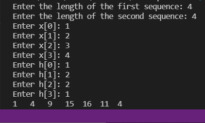
Enter the length of the first sequence: 4
Enter the length of the second sequence: 4
Enter x[0]: 1
Enter x[1]: 2
Enter x[2]: 3
Enter x[3]: 4
Enter h[0]: 1
Enter h[1]: 2
Enter h[2]: 2
Enter h[3]: 1

Output:

1 4 9 15 16 11 4

👁 Output