Articulation Points (or Cut Vertices) in a Graph

Given an undirected graph consisting of V vertices and E edges. The graph is represented as a 2D array edges[][], where each element edges[i] = [u, v] denotes an undirected edge between vertices u and v.
Find all the articulation points in the graph. If no such points exist, return {-1}.

An articulation point is a vertex whose removal, along with all its connected edges, increases the number of connected components in the graph.

Note: The graph may be disconnected, meaning it can consist of multiple connected components.

Examples:

Input: V = 5, edges[][] = [[0, 1], [1, 4], [4, 3], [4, 2], [2, 3]]

👁 1

Output: [1, 4]
Explanation: Removing vertex 1 or 4 disconnects the graph, as illustrated below:

👁 2

Input: V = 4, edges[][] = [[0, 1], [0, 2]]
Output: [0]
Explanation: Removing the vertex 0 will increase the number of disconnected components to 3.

[Naive Approach] - Using DFS - O(V × (V + E)) Time and O(V) Space

The idea is to traverse all the vertices and check whether it could be an articulation point or not. For that, remove the chosen vertex and call DFS (Depth First Search) on its neighbors. If DFS needs to be called more than once (i.e., multiple disconnected components are formed), then removing that vertex increases the number of components, so it is an articulation point.

1 4 

[Better Approach] - Using Tarjan's Algorithm - O(V + E) Time and O(V) Space

The idea is to use DFS to track how each node connects to its ancestors using discovery time and low values. Here, discovery time records when a node is first visited, and the low value represents the earliest (smallest) discovery time reachable from that node, including via back edges. For every node, we try to determine whether its subtree has an alternative path to reach an ancestor. If such a path does not exist for a child subtree, then the current node becomes a critical connection point, and removing it would disconnect that subtree from the rest of the graph. By propagating these low values during DFS, we can efficiently identify all nodes whose removal increases the number of connected components, i.e., the articulation points.

Let's understand with an example:

👁 example-1drawio

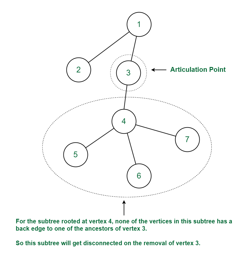
For the vertex 3 (which is not the root), vertex 4 is the child of vertex 3. No vertex in the subtree rooted at vertex 4 has a back edge to one of ancestors of vertex 3. Thus on removal of vertex 3 and its associated edges the graph will get disconnected or the number of components in the graph will increase as the subtree rooted at vertex 4 will form a separate component. Hence vertex 3 is an articulation point.

Now consider the following graph:
👁 Tree1drawio

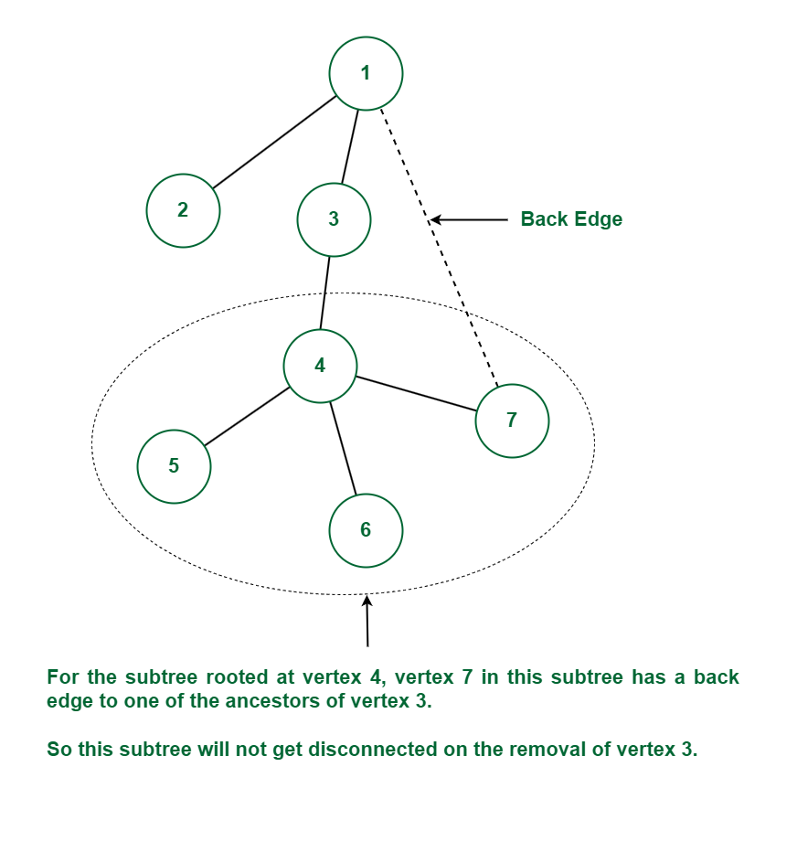
Again the vertex 4 is the child of vertex 3. For the subtree rooted at vertex 4, vertex 7 in this subtree has a back edge to one of the ancestors of vertex 3 (which is vertex 1). Thus this subtree will not get disconnected on the removal of vertex 3 because of this back edge. Since there is no child v of vertex 3, such that subtree rooted at vertex v does not have a back edge to one of the ancestors of vertex 3. Hence vertex 3 is not an articulation point in this case.

Step by Step implementation:

Maintain these arrays and integers and perform a DFS traversal.

• disc[]: Discovery time of each vertex during DFS.
• low[]: The lowest discovery time reachable from the subtree rooted at that vertex (via tree or back edges).
• parent: To keep track of each node’s parent in the DFS tree.
• visited[]: To mark visited nodes.

Root Node Case:

• For the root node of DFS (i.e., parent[u] == -1), check how many child DFS calls it makes.
• If the root has two or more children, it is an articulation point

For any non-root node u, check all its adjacent nodes:

• If v is an unvisited child, recur for v, and after returning update low[u] = min(low[u], low[v]) .
• If low[v] >= disc[u], then u is an articulation point because v and its subtree cannot reach any ancestor of u, so removing u would disconnect v.

Back Edge Case

• If v is already visited and is not the parent of u then It’s a back edge. Update low[u] = min(low[u], disc[v])
• This helps bubble up the lowest reachable ancestor through a back edge.

After DFS traversal completes, all nodes marked as articulation points are stored in result array.

1 4 

[Expected Approach] - Using Tarjan’s Algorithm (Iterative Method) - O(V + E) Time and O(V) Space

We can use Tarjan’s algorithm with an explicit stack to manage the traversal state instead of relying on the system’s call stack. The logic remains the same that we maintain disc, low, parent, and childrenCount but we manually control how nodes are processed.

For each node, we store its current state, including which neighbor to visit next and whether the node is in the entering or exiting phase.

With this approach, we preserve the core idea of Tarjan’s algorithm while making it more suitable for large or deep graphs.

1 4