Ford-Fulkerson Algorithm for Maximum Flow Problem

The Ford-Fulkerson algorithm is a widely used algorithm to solve the maximum flow problem in a flow network. The maximum flow problem involves determining the maximum amount of flow that can be sent from a source vertex to a sink vertex in a directed weighted graph, subject to capacity constraints on the edges.

The algorithm works by iteratively finding an augmenting path, which is a path from the source to the sink in the residual graph, i.e., the graph obtained by subtracting the current flow from the capacity of each edge. The algorithm then increases the flow along this path by the maximum possible amount, which is the minimum capacity of the edges along the path.

Problem:

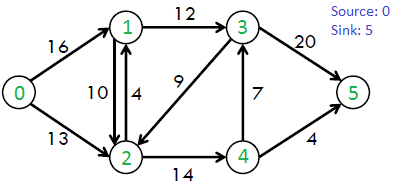
Given a graph which represents a flow network where every edge has a capacity. Also, given two vertices source 's' and sink 't' in the graph, find the maximum possible flow from s to t with the following constraints:

• Flow on an edge doesn't exceed the given capacity of the edge.
• Incoming flow is equal to outgoing flow for every vertex except s and t.

For example, consider the following graph from the CLRS book. 

👁 ford_fulkerson1

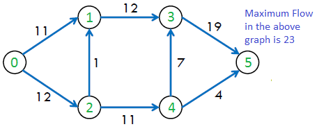
The maximum possible flow in the above graph is 23. 

👁 ford_fulkerson2

Prerequisite : Max Flow Problem Introduction

Ford-Fulkerson Algorithm 

 The following is simple idea of Ford-Fulkerson algorithm:

1. Start with initial flow as 0.
2. While there exists an augmenting path from the source to the sink:  
   • Find an augmenting path using any path-finding algorithm, such as breadth-first search or depth-first search.
   • Determine the amount of flow that can be sent along the augmenting path, which is the minimum residual capacity along the edges of the path.
   • Increase the flow along the augmenting path by the determined amount.
3. Return the maximum flow.

Time Complexity: Time complexity of the above algorithm is O(max_flow * E). We run a loop while there is an augmenting path. In worst case, we may add 1 unit flow in every iteration. Therefore the time complexity becomes O(max_flow * E).

How to implement the above simple algorithm? 
Let us first define the concept of Residual Graph which is needed for understanding the implementation. 

Residual Graph of a flow network is a graph which indicates additional possible flow. If there is a path from source to sink in residual graph, then it is possible to add flow. Every edge of a residual graph has a value called residual capacity which is equal to original capacity of the edge minus current flow. Residual capacity is basically the current capacity of the edge. 

Let us now talk about implementation details. Residual capacity is 0 if there is no edge between two vertices of residual graph. We can initialize the residual graph as original graph as there is no initial flow and initially residual capacity is equal to original capacity. To find an augmenting path, we can either do a BFS or DFS of the residual graph. We have used BFS in below implementation. Using BFS, we can find out if there is a path from source to sink. BFS also builds parent[] array. Using the parent[] array, we traverse through the found path and find possible flow through this path by finding minimum residual capacity along the path. We later add the found path flow to overall flow. 

The important thing is, we need to update residual capacities in the residual graph. We subtract path flow from all edges along the path and we add path flow along the reverse edges We need to add path flow along reverse edges because may later need to send flow in reverse direction (See following link for example).
https://www.geeksforgeeks.org/dsa/max-flow-problem-introduction/

Below is the implementation of Ford-Fulkerson algorithm. To keep things simple, graph is represented as a 2D matrix. 

The maximum possible flow is 23

Time Complexity : O(|V| * E^2) ,where E is the number of edges and V is the number of vertices.

Space Complexity :O(V) , as we created queue.

The above implementation of Ford Fulkerson Algorithm is called . The idea of Edmonds-Karp is to use BFS in Ford Fulkerson implementation as BFS always picks a path with minimum number of edges. When BFS is used, the worst case time complexity can be reduced to O(VE²). The above implementation uses adjacency matrix representation though where BFS takes O(V²) time, the time complexity of the above implementation is O(EV³) (Refer for proof of time complexity)

This is an important problem as it arises in many practical situations. Examples include, maximizing the transportation with given traffic limits, maximizing packet flow in computer networks.
Dinc's Algorithm for Max-Flow.

Exercise: 
Modify the above implementation so that it that runs in O(VE²) time.