 |
VOOZH | about |
|
VOOZH | about |
Dynamic Programming (DP) is a method used to solve complex problems by breaking them into smaller overlapping subproblems and storing their results to avoid recomputation. It is an optimization technique that transforms recursive solutions with exponential time into efficient ones with polynomial time.
When we try to solve complex problems, especially those involving choices or sequences, we often notice that the same smaller problems appear again and again. If we solve them every time from scratch, it leads to unnecessary repetition and wasted computation.
Dynamic Programming helps us avoid this. Instead of recomputing results, we remember (or store) the solutions of smaller problems and reuse them when needed.
This simple idea — of remembering the past to solve the future faster — forms the core of DP.
Dynamic Programming is a commonly used algorithmic technique used to optimize recursive solutions when same subproblems are called again.
Dynamic programming is used for solving problems that consists of the following characteristics:
The property Optimal substructure means that we use the optimal results of subproblems to achieve the optimal result of the bigger problem.
Example:
Consider the problem of finding the minimum cost path in a weighted graph from a source node to a destination node. We can break this problem down into smaller subproblems:
- Find the minimum cost path from the source node to each intermediate node.
- Find the minimum cost path from each intermediate node to the destination node.
The solution to the larger problem (finding the minimum cost path from the source node to the destination node) can be constructed from the solutions to these smaller subproblems.
The same subproblems are solved repeatedly in different parts of the problem refer to Overlapping Subproblems Property in Dynamic Programming.
Example:
Consider the problem of computing the Fibonacci series. To compute the Fibonacci number at index n, we need to compute the Fibonacci numbers at indices n-1 and n-2. This means that the subproblem of computing the Fibonacci number at index n-2 is used twice (note that the call for n - 1 will make two calls, one for n-2 and other for n-3) in the solution to the larger problem of computing the Fibonacci number at index n.
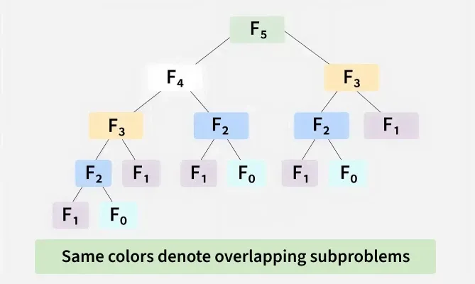
You may notice overlapping subproblems highlighted in the second recursion tree for Nth Fibonacci diagram shown below.
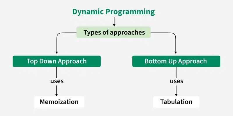
Dynamic programming can be achieved using two approaches:
In the top-down approach, also known as memoization, we keep the solution recursive and add a memoization table to avoid repeated calls of same subproblems.
In the bottom-up approach, also known as tabulation, we start with the smallest subproblems and gradually build up to the final solution.
Please refer Tabulation vs Memoization for the detailed differences.
Example 1: Consider the problem of finding the Fibonacci sequence:
Fibonacci sequence: 0, 1, 1, 2, 3, 5, 8, 13, 21, 34, ...
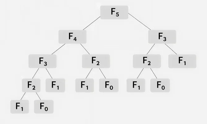
Brute Force Approach: To find the nth Fibonacci number using a brute force approach, you would simply add the (n-1)th and (n-2)th Fibonacci numbers.
5
Below is the recursion tree of the above recursive solution.
The time complexity of the above approach is exponential and upper bounded by O(2n) as we make two recursive calls in every function.
Let us now see the above recursion tree with overlapping subproblems highlighted with same color. We can clearly see that that recursive solution is doing a lot work again and again which is causing the time complexity to be exponential. Imagine time taken for computing a large Fibonacci number.
To achieve this in our example we simply take an memo array initialized to -1. As we make a recursive call, we first check if the value stored in the memo array corresponding to that position is -1. The value - 1 indicates that we haven't calculated it yet and have to recursively compute it. The output must be stored in the memo array so that, next time, if the same value is encountered, it can be directly used from the memo array.
5
In this approach, we use an array of size (n + 1), often called dp[], to store Fibonacci numbers. The array is initialized with base values at the appropriate indices, such as dp[0] = 0 and dp[1] = 1. Then, we iteratively calculate Fibonacci values from dp[2] to dp[n] by using the relation dp[i] = dp[i-1] + dp[i-2]. This allows us to efficiently compute Fibonacci numbers in a loop. Finally, the value at dp[n] gives the Fibonacci number for the input n, as each index holds the answer for its corresponding Fibonacci number.
5
In the above code, we can see that the current state of any fibonacci number depends only on the previous two values. So we do not need to store the whole table of size n+1 but instead of that we can only store the previous two values.
5
Dynamic programming has a wide range of advantages, including:
Dynamic programming has a wide range of applications, including: