Mason's Gain Formula in Control System

Mason's Gain Formula, also known as Mason's Rule or the Signal Flow Graph Method, is a technique used in control systems and electrical engineering. It provides a systematic way to analyze the transfer function of a linear time-invariant (LTI) system, especially those with multiple feedback loops and complex interconnections.

• Mason’s Gain Formula (MGF) helps determine the transfer function of a linear signal flow graph.
• Total gain represents the relationship between input variables and output variables in a system.
• Signal labeling allows formation of equations that describe relationships among different signals.
• Solving those equations expresses the output signal in terms of the input signal.

Mason's Gain Formula

Mason's gain formula for the determination of the overall system gain is given by:

where,

N: total number of forward paths

P_i : gain of the i^th forward path

∆: determinant of the graph

∆_i : path-factor for the i^th path

The determinant of the graph (∆) and the path-factor for the i^th path (∆_i) are defined as follows:

∆_i : 1 - (loop gain which does not touch the forward path)

∆: 1 - Σ(all individual loop gains) + Σ(gain product of all possible combinations of two non-touching loops) - Σ(gain product of all possible combinations of three non-touching loops) + ....

Important Terminologies of Mason's Gain Formula

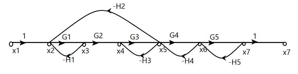
• Path: Traversal along connected branches where no node appears more than once.
• Forward Path: Traversal from the input node to the output node.
• Forward Path Gain: Product of all branch gains encountered along a forward path.
• Loop: Closed path that begins and ends at the same node.
• Non Touching Loops: Loops that do not share any common node.
• Loop Gain: Product of branch gains along a closed loop.

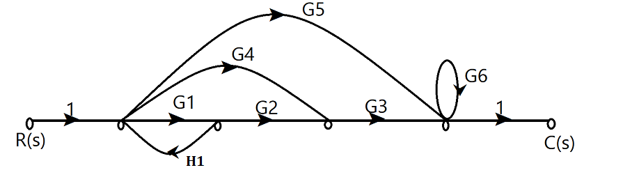
Let us consider a signal flow graph for understanding the above elements:

Forward Path

Form the above signal flow graph (SFG) image, there are two forward paths with their path gain as:

• P1 = ACEH
• P2 = AGH

Loop

There are 4 individual loops in the above SFG with their loop gain as:

• L1 = BC
• L2 = EHD
• L3 = F
• L4 = GHDB

Non-Touching Loops

There are ONE possible combinations of the non-touching loop with loop gain product as -

• L1.L3 = BCF

In above SFG, there are no combinations of three non-touching loops, 4 non-touching loops and so on.

Where,

• ∆₁ = 1 (since all loops are touching P₁)
• ∆₂ = 1 (since all loops are touching p2)
• ∆ = 1- [L1+L2+L3+L4] + [L1.L3]
• ∆=1 - (BC + EHD + F + GHDB) + BCF

Transfer Function:

Solved Examples on Mason Gain Formula

Example 1: Find the transfer function of the following signal flow graph

Solution:

No. of forward path(N) = 1

Gain of Forward Paths (P1) = 1*G1G2G3G4G5

No. of individual loops:

• L1 = -G1H1
• L2 = -G3H3
• L3 = -G4H4
• L4 = -G5H5
• L5 = -G1G2G3H2

Non-Touching Loops (Combination of two):

• L1L2 = G1G3H1H3
• L1L3 = G1G4H1H4
• L1L4 = G1G5H1H5
• L24 = G3G5H3H5
• L4L5 = G1G2G3G5H2H5

Non-Touching Loops (Combination of three):

• L1L2L4 = -G1G3G5H1H3H5
  

Here,

∆₁ = 1 (since all loops are touching p1)

∆ = 1 - (L1+L2+L3+L4+L5) + (L1L2+L1L3+L1L4+L2L4+L4L5) - (L1L2L4)

Transfer Function:

Example 2: Find the transfer function of the following signal flow graph

Solution:

There are two forward paths and one loop. So, we have

• P₁ = a
• P₂ = b
• L₁ = c
• ∆₁ = ∆₂ = 1 (since all loops are touching P₁ & P₂)
• ∆ = 1 - c

Transfer Function:

Example 3: Find the transfer function of the following signal flow graph

No. of forward path(N) = 3

The gain of Forward Paths:

1. P1 = G1G2G3
2. P2 = G4G3
3. P3 = G5

No. of individual loops:

• L1 = G1H1
• L2 = G6

Non-Touching Loops (Combination of two)

• L1L2 = G1G6H1

∆₁ = ∆₂ = ∆₃ = 1 (since all loops are touching P1,P2 &P3)

∆ = 1 - (G1H1+G6) + G1G6H1

Transfer Function:

Advantages & Disadvantages

Advantages

• Simplicity: A systematic procedure helps in calculating overall gain of a complex control system.

• Comprehensive: Analysis remains possible even when several feedback loops exist in a system.

• Versatility: Usage remains suitable for linear time-invariant control systems.

• Visualization: Identification of different paths and loops becomes easier, which improves understanding of system behaviour.

Disadvantages

• Complexity for Large Systems: Large numbers of loops and paths increase calculation difficulty and time.

• Limited to Linear Systems:Application mainly focuses on linear time-invariant systems and does not directly support nonlinear or time-varying systems.

• Assumption of Non Touching Loops: Analysis assumes loops do not intersect, which may not match some practical systems.

• Limited Practical Insight: Calculation focuses on overall gain and may not clearly explain stability or dynamic characteristics required in some applications.

Applications

• Stability Analysis: Calculation of poles and zeros of the overall transfer function helps in studying system stability.

• Closed-Loop Systems: Evaluation of feedback effects helps in understanding overall system performance.

• Transient and Steady-State Response: Study of system behaviour for transient conditions and steady-state inputs becomes easier.

• Filter Design: Analysis of frequency response supports the design and development of filters.