Nyquist Plot

A Nyquist plot is a graphical representation used in control engineering. It is used to analyze the stability and frequency response of a system. The plot represents the complex transfer function of a system in a complex plane. The x-axis represents the real part of the complex numbers and the y-axis represents the imaginary part. Each point on the Nyquist plot reflects the complex value of the transfer function at that frequency.

Nyquist Stability Criteria

It is used to determine the stability of a control system. This criterion works on the principle of argument. It is useful for feedback control system analysis and is expressed in terms of frequency domain plot. It is applicable for minimum and non-minimum phase systems.

👁 Nyquist-Plot

According to the Nyquist Stability Criterion the number of encirclement of the point (-1, 0) is equal to the P-Z times of the closed loop transfer function. The equation for stability analysis is given below:

N = Z - P ------ (equation 1)

Where,
P = open loop pole of the system on right hand side (RHP)
Z = close loop zero of the system on right hand side (RHP)
N = number of encirclement around (-1,0)

Note: 'N' is negative for anticlockwise encirclement around (-1,0) and positive for clockwise encirclement around (-1,0).

Stability Cases:

N (encirclements)	Condition	Stability
0 (no encirclement)	Z = P = 0 $ Z = P	Marginally stable
N > 0 (clockwise encirclement)	P = 0, Z ≠0 & Z > P	Unstable
N < 0 (anti-clockwise encirclements)	Z = 0, P ≠0 & P > Z	Stable

Principle of Argument in Nyquist Plot

It states that if in a transfer function, there are 'P' poles and 'Z' zeros enclosed in s-plane contour, then the corresponding GH plane contour will encircle the origin 'Z-P' times as seen in equation 1.

• If the contour encircles more zeros than poles (Z > P), there is increase in the encirclement number which leads to a positive value of N. This corresponds to a clockwise encirclement of the critical point, indicating instability.
• If the contour encircles more poles than zeros (P > Z), there is decrease in encirclement number which leads to a negative value of N. This corresponds to a anti-clockwise encirclement of the critical point, indicating stability.
• If the number of poles and zeros enclosed by the contour are equal (Z = P), the encirclement number is zero, indicating a marginally stable system. The contour neither contributes to a net clockwise nor counter-clockwise encirclement.

Important Terminologies of Nyquist Plot

Important terminologies of Nyquist Plot are mentioned below:

• Nyquist Path or Contour
• Nyquist Encirclement
• Nyquist Mapping
• Gain Crossover Frequency
• Phase cross over frequency
• Phase Margin
• Gain Margin

1. Nyquist Path or Contour

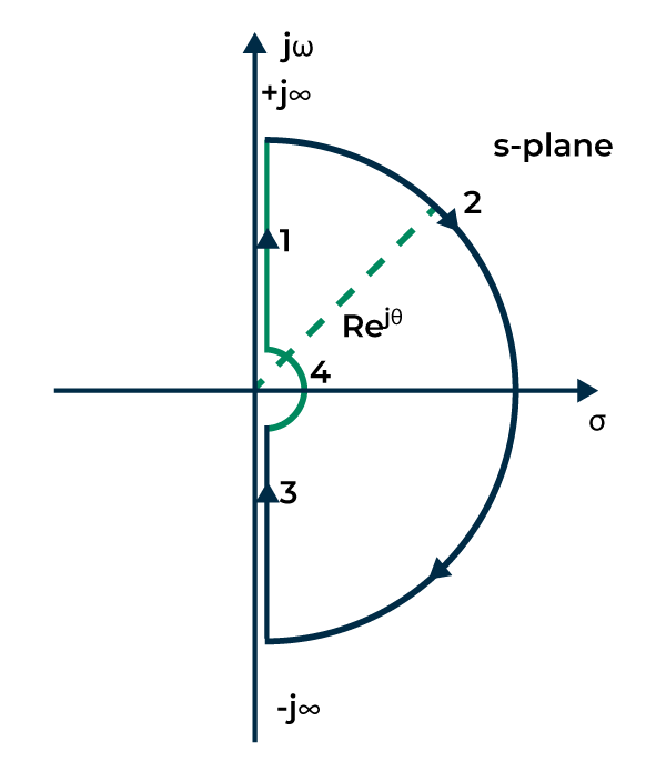
The Nyquist Path or Contour is a closed contour on the right side of the s-plane. To enclose the entire RHS of the plane, a large semicircle lane is drawn with a diameter along the 'j' axis and center at the source. The semicircle radius is simply treated as Nyquist Encirclement. The Nyquist Contour is shown in the figure below:

👁 Nyquist-Plot-1

In the above plot, marked points are denoting:

Point 1 is denoting s = jω
Point 2 is denoting s = where, θ = +90^o to -90^o
Point 3 is denoting s = -jω
Point 2 is denoting s = where, θ = -90^o to +90^o

2. Nyquist Encirclement

It is a point, if it is found in the curve, is known to be encircled by a line.

3. Nyquist Mapping

Mapping is the process of transforming a point in the s-plane into a point in the F(s) plane, and F(s) is the result of mapping.

4. Gain Crossover Frequency

It is the frequency at which the Nyquist plot has unity magnitude. It is denoted by 'ω_gc'.

5. Phase cross over frequency

It is the frequency at which point the Nyquist plot crosses the negative real axis is called the phase cross-over frequency and it is denoted with 'ω_pc'.

6. Phase Margin

The phase margin indicates how much more phase shift we may put in the open loop transfer function before our system becomes unstable. It can be calculated from the phase at the gain cross-over frequency.

7. Gain Margin

The gain margin is the amount of open loop gain that can be increased before our system becomes unstable. It can be calculated from the gain at the phase cross-over frequency.

How to Draw Nyquist Plot?

Procedure to draw Nyquist Plot:

1. Draw Polar Plot
2. Draw Inverse polar Plot
3. Draw and map using Nyquist Contour

Rules of Nyquist Plot

1. Determine the transfer function of the system.
2. Calculate the complex transfer function value by putting s= jω, where 'ω' is angular frequency and 'j' is the imaginary unit.
3. Determine the magnitude and phase of the complex transfer function.
4. Plot the points in the polar coordinate for each frequency point.
5. Connect all the points to create a smooth Nyquist curve. The curve represents the change in magnitude and phase with frequency.
6. Calculate the number of encirclements around the point (-1,0). Each encirclement represents the value of 'N'. The stability can be calculated using Nyquist Stability Criteria as discussed above.

Stability Analysis Using Nyquist Plot

The nyquist plot helps in analysis of the stability of a control system. It tells whether the system is stable, unstable or marginally stable. The stability is analyzed using various parameters which are as follows:

• Gain cross-over frequency
• Phase cross-over frequency
• Gain margin
• Phase margin

Phase Cross Over Frequency

It is the frequency at which point the Nyquist plot crosses the negative real axis is called the phase cross-over frequency and it is denoted with 'ω_pc'.

The stability of the control system based on the relationships between the two frequencies i.e., phase cross-over and gain cross-over is given below:

ωpc > ωgc ->System is stable

ωpc < ωgc ->System is unstable

ωpc = ωgc ->System is marginally stable

Phase Margin

The phase margin indicates how much more phase shift we may put in the open loop transfer function before our system becomes unstable. It can be calculated from the phase at the gain cross-over frequency.

Phase Margin (PM) = 180^∘+∠G(jω)H(jω)∣_ω=ωgc

The stability of the control system based on the relationships between the two margins i.e., gain margin and phase margin is given below:

GM > 1 and PM is positive -> System is stable

GM < 1 and PM is negative ->System is unstable

GM = 1 and PM is 0^o ->System is marginally stable

Gain Crossover Frequency

It is the frequency at which the Nyquist plot has unity magnitude. It is denoted by 'ω_gc'.

Gain Margin

The gain margin is the amount of open loop gain that can be increased before our system becomes unstable. It can be calculated from the gain at the phase cross-over frequency.

Gain Margin (GM):

Let us understand the above concept with the help of an example.

Question: Find the gain crossover frequency and phase margin of the given transfer function

Solution

PM = 180^∘+∠G(jω)H(jω)∣_ω=ωgc

ω_gc = Frequency at which magnitude of G(s)H(s) is equal to 1.

G(jω)H(jω) =

|G(jω)H(jω)| = 1

= 1

On solving the quadratic equation we will get:

ω_gc = (we will neglect the negative term inside the root)

ω_gc will now become =

ω_gc = 0.786 rad/sec

Now finding the phase at gain crossover frequency

∠G(jω)H(jω)∣_ω=ωgc = - tan^-1 (ω_gc)

∠G(jω)H(jω)∣_ω=ωgc = - tan^-1 (0.786)

∠G(jω)H(jω)∣_ω=ωgc = -90^o - 38.16^o

∠G(jω)H(jω)∣_ω=ωgc = -128.16

PM = 180 - 128.16

PM = 51.84^o

Solved Example of Nyquist Plot

1. Draw the Nyquist plot for the system whose open loop transfer function is given by

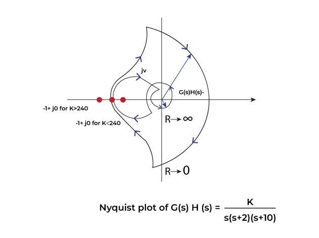
G(s)H(s) =

Also determine the value of 'k' for which the system is stable.

Solution

Step 1: Identify the poles and zeros

There are 3 poles and no zeros

Poles: 0, -2, -10

G(s)H(s) =

Step 2: Mapping of all the 4 section as seen in the given image

👁 Nyquist-Plot-1

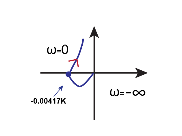
The value of ω in the region (1) is s = jω. Replacing the transfer function with s = jω

G(jω)H(jω) =

G(jω)H(jω) =

G(jω)H(jω) = ----- equation 1

Now keeping the imaginary term 0 to find the phase crossover frequency.

ω(1 - 0.05ω²) = 0

1 - 0.05ω² = 0

ω = 4.472 = phase crossover frequency

Putting the value of frequency in the real part of the equation 1.

G(jω)H(jω) =

G(jω)H(jω) =

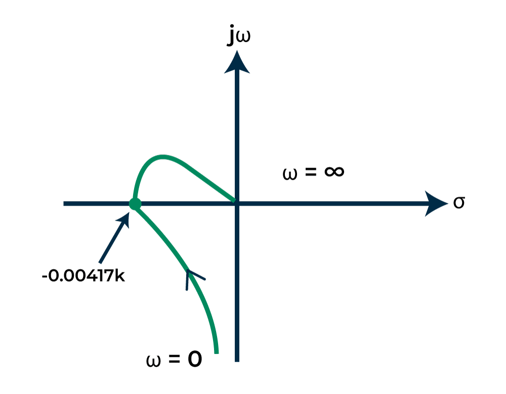
G(jω)H(jω) = -0.00417K

The polar plot will start at -90 degrees and crosses the x axis at point -0.00417K as given below:

👁 Nyquist-Plot-new

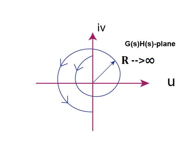
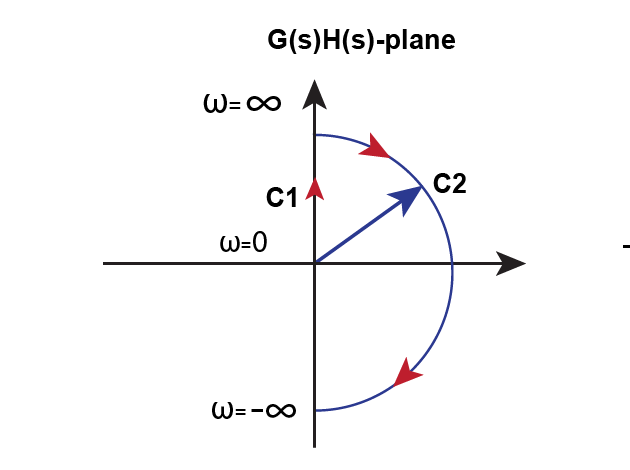
Step 3: Mapping the region 2 whose equation is given by: s = where, θ = +90^o to -90^o

If the transfer function is in the form G(s)H(s) = , then assume that (1 + sT) is equal to sT. It is given by:

G(s)H(s) =

G(s)H(s) =

G(s)H(s) =

Let s =

G(s)H(s) =

At , G(s)H(s) =

At , G(s)H(s) =

Thus, the region 2 varies from -270 degrees to 270 degrees. It is represented below:

👁 Nyquoist-Pl-03

Step 4: Now map the region 3 of the nyquist contour. The region 3 is simple inverse of region 1. Thus the graph will mirror image of region 1 graph which is shown below:

👁 Nyquoist-Pl-04

Step 5: Mapping the region 4 whose equation is given by: s = ,where, θ = -90^o to +90^o

If the transfer function is in the form G(s)H(s) = , then assume that (1 + sT) is equal to 1. It is given by:

G(s)H(s) =

G(s)H(s) =

Let s = s =

G(s)H(s) = ∞

At , G(s)H(s) = ∞

At , G(s)H(s) = ∞

So the graph will be circular arc of infinite radius as seen in the given image.

👁 Nyquoist-Pl-05

Step 6: Now we will perform the stability analysis. To find the value of 'k', we will check when our contour will pass through the point (-1+j0)

-0.00417K = -1

K = 1/0.00417

K = 240

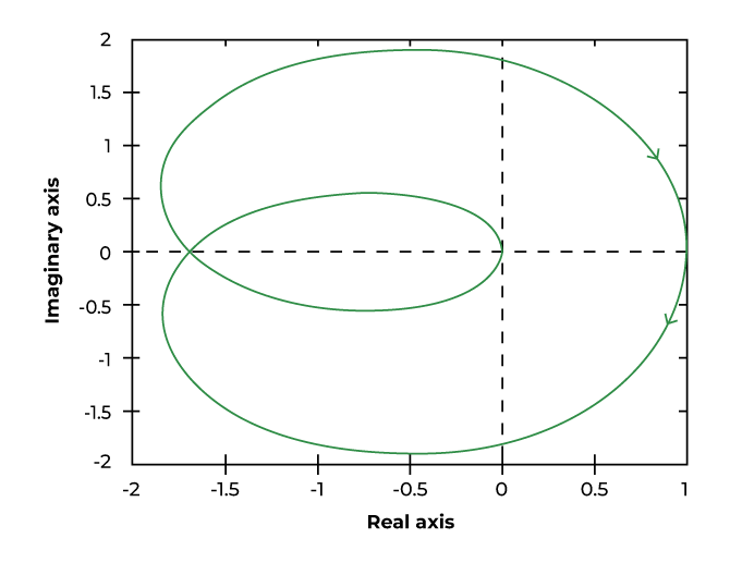
Step 7: Final Nyquist Plot is shown below. It as been plotted by combining the mapping of all the four regions.

👁 Nyquoist-Pl-06

Now we will check foe which value of 'k', the system is stable.

Case 1: If k< 240

The point -1+j0 is not encircled. This means that there are no poles on the right half of the plane. This means the system is stable for k less than 240.

Case 2: k>240

The point -1+j0 is encircled two times in the clockwise direction. This means that Z>P and hence the system is unstable.

Stability condition: 0 < K < 240

Advantages of Nyquist Plot

1. It provides a graphical representation of the system that how a system responds to different frequencies.
2. It simplifies the calculation of the stability of a system without calculating the poles explicitly.
3. It provides the number of unstable poles in the closed loop system by just calculating the encirclements around critical points.
4. It helps in adjusting the parameters like gain and phase margins to achieve stability.
5. It is useful to analyze the stability and behavior of the feedback control system.

Disadvantages of Nyquist Plot

1. It is very time consuming to draw it by hand and more prone to errors with complex transfer function.
2. It is applicable to LTI system. It cannot be applied to non-linear or time varying systems.
3. It rely on open-loop transfer function and can lead to inaccurate representation of the behavior of closed-loop system.
4. It does not provide the information about transient response.

Application of Nyquist Plot

• Stability analysis: It is used in stability analysis of a control system by determining the number of encirclements around a specific point.

• Control system design: It is used in adjusting the controller parameters like gain margins and phase margins to achieve the desired stability of a control system.

• Phase margin evaluation: It represents the system's robustness and stability margin. It can be directly read from the plot and can be adjusted accordingly to achieve the stability.

• Filter designing: It is used in the design of filters and equalizers to optimize frequency response and phase characteristics for desired signal processing applications.

• Feedback loop analysis: It is used in the analysis of the feedback loops which affect the stability and performance of a control system. It shows that how change in controller or system parameters influence the overall behavior.