Solve Interview Case Studies 10x Faster Using Dynamic Programming

Introduction

The ability to solve case studies comes with regular practice. Many a times, if you find yourself failing at thinking like a pro, perhaps, it’s just because you haven’t practiced enough.

To help you become confident, I’ve written multiple case studies in last one month. You can check the recent ones here. If you haven’t solved any of them, I’d suggest you to check them out first.

Dynamic Programming a.k.a Dynamic Optimization isn’t any trick or a mathematical formula which delivers correct answer just by providing the inputs. Rather, it’s a combination of structured thinking & analytical mindset which does the job. The concept is an old one, yet used by just few of us.

In this article, I have explained the art of dynamic programming using a Taxi-Replacement case study. The case study is meant for advanced users. Also, I’ve used R to implement dynamic programming so that, you get some real coding experience as well.

For freshers, I’d recommend checking out the previous case study before trying their hand at this one. And if you truly want to land your first data science role, you can’t go wrong with the ‘Ace Data Science Interviews‘ course. Start your data science journey today! 

👁 analytics case studies using dynamic programming

Case Study –  Taxi Replacement

Assume, you’ve decided to start a Taxi Operator firm. In fact, you’ve a meeting scheduled with top investors next week. For which, you need to present your business plan. The focus of your plan should be the amount of revenue expected year on year for next 25 years and your growth strategy.

A critical decision which can set you for success is to consider / estimate the time to change the cars. You know, you can’t operate on a taxi forever. Precisely, a car (taxi) cannot be used for more than 10 years. Also, you are not allowed to buy a used car.

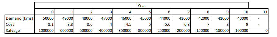
You plan to run 100 cars in total, however doing calculations for a single car will suffice. Here are the assumptions you need to make in this case study :

👁 assumptions1
Cost (INR/Km)

The salvage value is the price of the used car (second hand) at the end of respective year. As you see, the demand of the car decreases as the car grows old. Also, the mileage of the car decreases over the years.

The initial car cost (as of now) is 100,000 INR. As you can see, the value of car depreciates to 0 INR in the 11th year. This is because a car is not allowed to be driven more than 10 years (national rules). In addition, you need to take into account the inflation of values as below :

1. Initial Cab fare : INR 12
2. Increase in salvage value of the car : 1%
3. Increase in cost of a brand new car :  5%
4. Growth in annual demand : 3%
5. Increase in Cab fare : 4%
6. Increase in Cost (Maintenance and fuel) : 2%

Let’s get started!

What is Dynamic Programming?

Dynamic programming/Optimization is a method for solving a complex problem by breaking it down into a collection of simpler subproblems, solving each of those subproblems just once, and storing their solutions – ideally, using a memory-based data structure. It is a widely known algorithm in Operation Research.

But today, we will try to use this technique to solve the problem at hand.

Solution

Let’s define a simple optimization function for the current problem. We are trying to optimize the profit in the current problem and profit is given as:

Profit(t) = Demand(t) * (Cab Fare(t)-Cost(t)) + Sell of flag * (NewCarCost - SalvageValue(t))

Total Profit = Profit(t) + Profit(t+) +Profit(t-)

Sell of flag is 1 if we decide to sell the car and 0 otherwise. You should notice that all the values in this function are dependent on time.  So, from where do we start solving this problem?

From the very last time point. The reason being, at the last time point, we do not have any dependency of future time points. For instance at the last time point (l), we know that

Profit(l) = Demand(l)*(Cab Fare(l)-Cost(l)) + Sell off flag * (NewCarCost - SalvageValue(l))

and,

Profit(l-1,l) =  Demand(l-1)*(CabFare(l-1) - Cost(l-1)) + Sell off flag *
(NewCarCost - SalvageValue(l-1)) + Max(Profit(l))

Max(Profit(l)) is the maximum value of Profit(l) for the decision variable “Sell off flag”

So on till..

Total Profit = Max(Profit(l)) + Max(Profit(l-1)) + ......+Max(Profit(1))

Problem at Hand

We can solve the problem at hand with the following R code :

#Basic Assumptions

> Demand <- c(50000,49000,48000,47000,46000,45000,44000,43000,42000,41000,40000)
> cost <- c(3.1,3.3,3.6,4,4.5,5,5.6,6.3,7,8,9)
> Salvage<-c(1000000,600000,500000,400000,350000,300000,250000,200000,150000,130000,100000,0)

#Inflation rates
> Salvagegrowth <- 1.01
> InitialCostgrowth <- 1.05
> Demandgrowth <- 1.03
> cabfaregrowth <- 1.04
> costinggrowth <- 1.02

#Build the function to do dynamic programming

> findpath <- function(time){
profit_sell <- matrix(0,time + 1,12)
profit_keep <- matrix(0,time + 1,12)
profit_sell[,12] <- -100000000000
profit_keep[,12] <- -100000000000
sell_keep_grid <- matrix("Keep",time + 1,11)
Demand <- Demand*(Demandgrowth)^time
Salvage[1] <- Salvage[1]* (InitialCostgrowth)^time
Salvage[2:11] <- Salvage[2:11]*(Salvagegrowth)^time
cabfare <- 12*(cabfaregrowth)^time
cost <- cost*(costinggrowth)^time
for (i in time:1){
Demand <- Demand/Demandgrowth
Salvage[1] <- Salvage[1]/InitialCostgrowth
Salvage[2:11] <- Salvage[2:11]/Salvagegrowth
cabfare <- cabfare/cabfaregrowth
cost <- cost/costinggrowth
Profit <- Demand*(cabfare - cost)
for (j in 1:11){
profit_sell[i,j] <- max(profit_sell[i+1,2],profit_keep[i+1,2])+ Profit[1] + Salvage[j] - Salvage[1]
profit_keep[i,j] <-max(profit_sell[i+1,j+1],profit_keep[i+1,j+1])+Profit[j]
sell_keep_grid[i,j] <- ifelse(profit_sell[i,j] > profit_keep[i,j],"Sell","Keep")
sell_keep_grid[i,j] <- ifelse(i < j,"N/A",sell_keep_grid[i,j])
}
}

Path <- rep("Keep",time)
num_years <- rep(0,time)

lookat <- 1
for(i in 1:time) {
Path[i] <- sell_keep_grid[i,lookat]
num_years[i] <- lookat
lookat <- ifelse(sell_keep_grid[i,lookat] == "Sell",1,lookat+1)
}
setwd("C:\\Users\\ts93856\\Desktop\\Insurance")
write.csv(profit_sell,"Sell.csv")
write.csv(profit_keep,"keep.csv")
write.csv(sell_keep_grid,"sellkeepgrid.csv")
write.csv(Path,"Path.csv")
print(num_years)
print(Path)
return(Path)
}

findpath(time = 25)

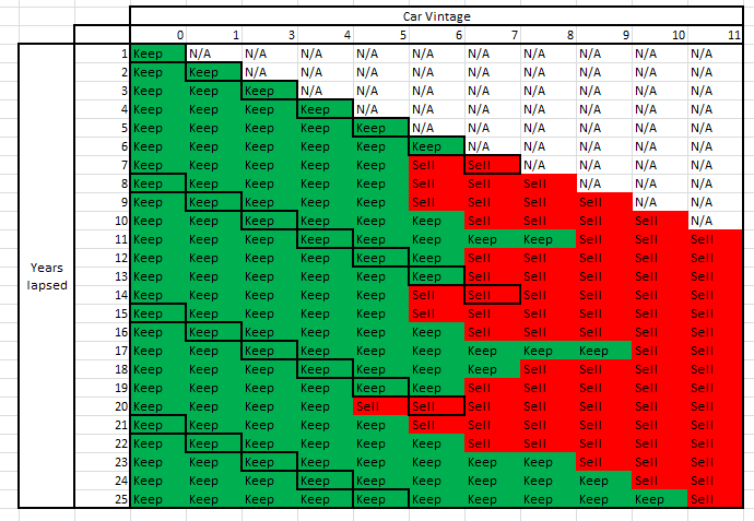
Here is the final output you get for Keep/Sell decision :

👁 result1

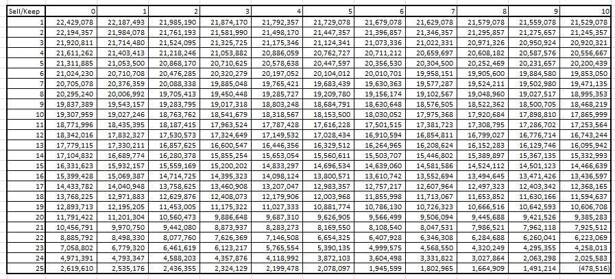
Further, let’s look at the Optimum revenue matrix :

👁 result2

As you can see, the total revenue in 1st cell is INR 22.4 Million which is the maximum profit expected by a single car in 25 years. Hence, the total expected profit by 100 cars will be 100*22.4 Million = INR 2.24 Billion based on our current assumptions.

Let’s try to answer a few more question using the same analysis.

Few more questions

Solved Questions:

1. What is the oldest car you will use in the most optimized combination?
2. In which year to expect the maximum profit (compare the present value assuming 6% inflation)?
3. What is the final salvage value of all 100 vehicles the company will have at the end of the 25 years? (Unsolved)

Solution

There are 4 cycles evident from the first table. So, we need 1 original and 3 replacements for each car requirement. The first car stays for 7 years, 2nd stays for 7 years, 3rd for 6 years and last for 5 years. So, the maximum age of the car here is 7 years.

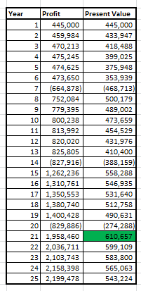
To find the year wise profit in present value, following is the table:

👁 result3

Hence, the maximum profit in present value happens at 21st year.

End Notes

I have left one of the question for you to practice the concept. This is one of the most powerful tools given by operation research domain to optimize such complex problems. You just saw, it isn’t any difficult to learn. You just need to put a framework around the give problems.

In future articles I will illustrate with more examples of how Dynamic Programming/Optimization is used in different industries. I’d recommend you to practice this technique so that you do well in your next job interview. All the best.

Did you like reading this article ?  Do share your experience / suggestions in the comments section below. I’d love to know your

You can test your skills and knowledge. Check out Live Competitions and compete with best Data Scientists from all over the world.

Login to continue reading and enjoy expert-curated content.

Free Courses