Anomaly detection is the process of finding abnormalities in data. Abnormal data is defined as the ones that deviate significantly from the general behavior of the data. Some of the applications of anomaly detection include fraud detection, fault detection, and intrusion detection. Anomaly Detection is also referred to as outlier detection.

Some of the anomaly detection algorithms are,

Local Outlier Factor
Isolation Forest
Connectivity Based Outlier Factor
KNN based Outlier Detection
One class SVM
AutoEncoders

Outlier Detection vs Novelty Detection

In outlier detection, the training data consists of both anomalies and normal observations whereas in novelty detection the training data consists only of normal observations rather than having both normal and anomalous observations. In this post, we’re gonna see a use case of novelty detection.

AutoEncoder

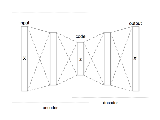
AutoEncoder is an unsupervised Artificial Neural Network that attempts to encode the data by compressing it into the lower dimensions (bottleneck layer or code) and then decoding the data to reconstruct the original input. The bottleneck layer (or code) holds the compressed representation of the input data. The number of hidden units in the code is called code size.

👁 Anomaly detection AutoEncoder

Image Source: https://commons.wikimedia.org/wiki/File:Autoencoder_structure.png

Applications of AutoEncoders

Dimensionality reduction
Anomaly detection
Image denoising
Image compression
Image generation

In this post let us dive deep into anomaly detection using autoencoders.

Anomaly Detection using AutoEncoders

AutoEncoders are widely used in anomaly detection. The reconstruction errors are used as the anomaly scores. Let us look at how we can use AutoEncoder for anomaly detection using TensorFlow.

Import the required libraries and load the data. Here we are using the ECG data which consists of labels 0 and 1. Label 0 denotes the observation as an anomaly and label 1 denotes the observation as normal.

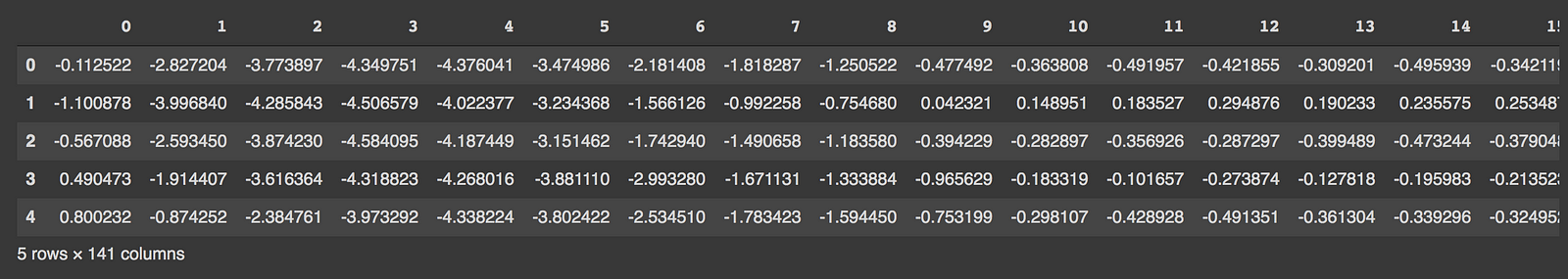
import numpy as np
import pandas as pd
import tensorflow as tf
import matplotlib.pyplot as plt
from sklearn.metrics import accuracy_score
from tensorflow.keras.optimizers import Adam
from sklearn.preprocessing import MinMaxScaler
from tensorflow.keras import Model, Sequential
from tensorflow.keras.layers import Dense, Dropout
from sklearn.model_selection import train_test_split
from tensorflow.keras.losses import MeanSquaredLogarithmicError

# Download the dataset
PATH_TO_DATA = 'http://storage.googleapis.com/download.tensorflow.org/data/ecg.csv'
data = pd.read_csv(PATH_TO_DATA, header=None)
data.head()

# data shape
# (4998, 141)

Output:

👁 Anomaly detection 1

# last column is the target
# 0 = anomaly, 1 = normal
TARGET = 140

features = data.drop(TARGET, axis=1)
target = data[TARGET]

x_train, x_test, y_train, y_test = train_test_split(
 features, target, test_size=0.2, stratify=target
)

# use case is novelty detection so use only the normal data
# for training
train_index = y_train[y_train == 1].index
train_data = x_train.loc[train_index]

# min max scale the input data
min_max_scaler = MinMaxScaler(feature_range=(0, 1))
x_train_scaled = min_max_scaler.fit_transform(train_data.copy())
x_test_scaled = min_max_scaler.transform(x_test.copy())

The last column in the data is the target ( column name is 140). Split the data for training and testing and scale the data using MinMaxScaler.

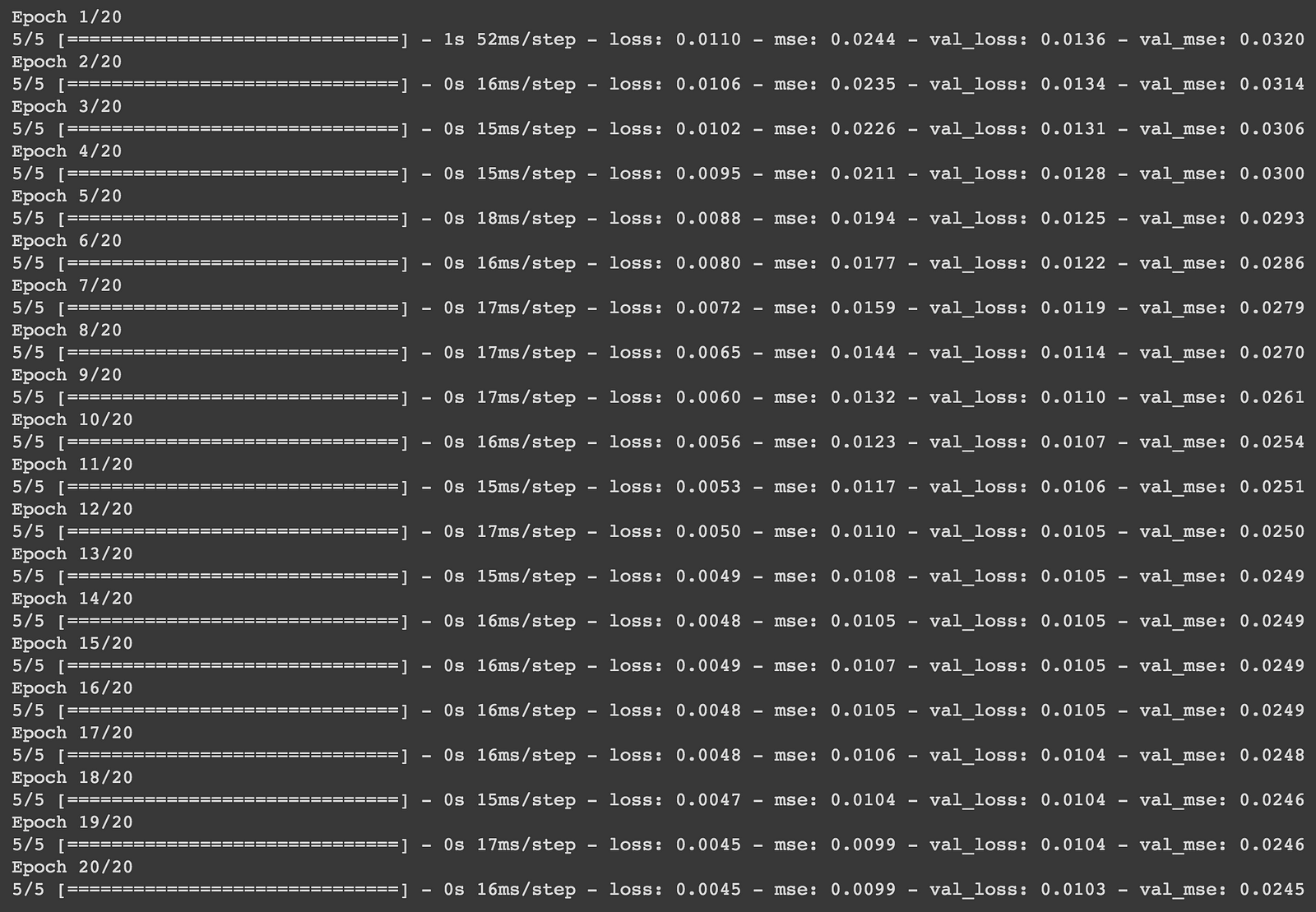
# create a model by subclassing Model class in tensorflow
class AutoEncoder(Model):
 """
 Parameters
 ----------
 output_units: int
 Number of output units
 
 code_size: int
 Number of units in bottle neck
 """

 def __init__(self, output_units, code_size=8):
 super().__init__()
 self.encoder = Sequential([
 Dense(64, activation='relu'),
 Dropout(0.1),
 Dense(32, activation='relu'),
 Dropout(0.1),
 Dense(16, activation='relu'),
 Dropout(0.1),
 Dense(code_size, activation='relu')
 ])
 self.decoder = Sequential([
 Dense(16, activation='relu'),
 Dropout(0.1),
 Dense(32, activation='relu'),
 Dropout(0.1),
 Dense(64, activation='relu'),
 Dropout(0.1),
 Dense(output_units, activation='sigmoid')
 ])
 
 def call(self, inputs):
 encoded = self.encoder(inputs)
 decoded = self.decoder(encoded)
 return decoded
 
model = AutoEncoder(output_units=x_train_scaled.shape[1])
# configurations of model
model.compile(loss='msle', metrics=['mse'], optimizer='adam')

history = model.fit(
 x_train_scaled,
 x_train_scaled,
 epochs=20,
 batch_size=512,
 validation_data=(x_test_scaled, x_test_scaled)
)

The encoder of the model consists of four layers that encode the data into lower dimensions. The decoder of the model consists of four layers that reconstruct the input data.

The model is compiled with Mean Squared Logarithmic loss and Adam optimizer. The model is then trained with 20 epochs with a batch size of 512.

👁 Anomaly detection Adam

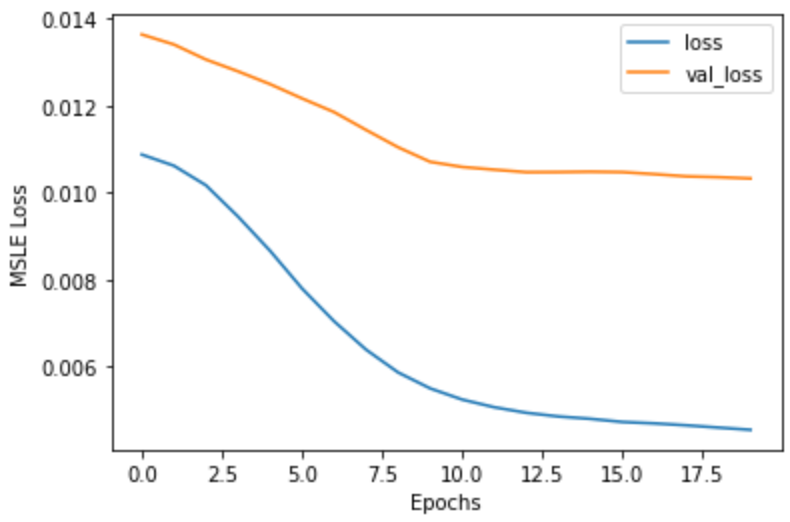
plt.plot(history.history['loss'])
plt.plot(history.history['val_loss'])
plt.xlabel('Epochs')
plt.ylabel('MSLE Loss')
plt.legend(['loss', 'val_loss'])
plt.show()

👁 Anomaly detection MSLE loss

def find_threshold(model, x_train_scaled):
 reconstructions = model.predict(x_train_scaled)
 # provides losses of individual instances
 reconstruction_errors = tf.keras.losses.msle(reconstructions, x_train_scaled)
 # threshold for anomaly scores
 threshold = np.mean(reconstruction_errors.numpy()) \
 + np.std(reconstruction_errors.numpy())
 return threshold

def get_predictions(model, x_test_scaled, threshold):
 predictions = model.predict(x_test_scaled)
 # provides losses of individual instances
 errors = tf.keras.losses.msle(predictions, x_test_scaled)
 # 0 = anomaly, 1 = normal
 anomaly_mask = pd.Series(errors) > threshold
 preds = anomaly_mask.map(lambda x: 0.0 if x == True else 1.0)
 return preds

threshold = find_threshold(model, x_train_scaled)
print(f"Threshold: {threshold}")
# Threshold: 0.01001314025746261
predictions = get_predictions(model, x_test_scaled, threshold)
accuracy_score(predictions, y_test)
# 0.944

The reconstruction errors are considered to be anomaly scores. The threshold is then calculated by summing the mean and standard deviation of the reconstruction errors. The reconstruction errors above this threshold are considered to be anomalies. We can further fine-tune the model by leveraging Keras-tuner.

The autoencoder model does not have to symmetric encoder and decoder but the code size has to be smaller than that of the features in the data.

Find the entire code in my Google Colab Notebook.