Understanding Gradient Descent Algorithm and the Maths Behind It

7 min read

This article throws light on how the Gradient Descent algorithm’s core formula is derived which will further help in better understanding of the Gradient Descent Algorithm. First, we will understand what is Gradient Descent algorithm is in brief.

This article was published as a part of the Data Science Blogathon

A Brief idea of Gradient Descent Algorithm

Imagine you are standing at a grassy park on a hill. Suppose you want to come down at the base of the hill as quickly as possible. So what would you do?

You will look around everywhere and think if you were to take baby steps in some direction to go downhill as quickly as possible then in what direction you will take those baby steps to walk down as rapidly as possible? You will find the best direction and take one step and land on a new point on the hill.

Again you will look around to find the direction to take the next baby step in order to go downhill. If you take that step, you will land upon another point on the hill.

This way thinking about what direction to go and take the step will be continued until you reach downhill which is the global minimum.

The Core of Gradient Descent Optimisation Algorithm

Gradient Descent is an Iterative Solver. The Iterative solver does not give the exact solution. Not in all cases, the objective function is solvable.

In such cases, the iterative solvers are used to get the approximate solution as the purpose is to minimize the objective function.

The basic principle of gradient descent is to choose the step size (also called as learning rate) appropriately so that we can get close to the exact solution. So learning rate basically controls how big a step we take downhill.

The gradient descent update rule is given as follows :

👁 update rule | Gradient descent algorithm

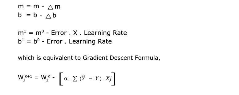
Gradient Descent can be summarized using the formula,

👁 weight update

_{Image Source: Created by Author}

We repeatedly calculate this until convergence.

Let’s see how we got this formula.

Also, you can Check Different types of Gradient Descent

Starting with a simple Machine Learning Model

We will take an example of a linear regression model.

Suppose you have a set of data points and a line in a 2-D space. If you plot these points and try to draw a line passing through these points, it will look like as follows :

_{Image Source: https://backlog.com/blog/gradient-descent-linear-regression-using-golang/}

The equation of a line is given as Y = mX + b where m is the slope of the line and b is the intercept on the Y-axis.

When you try to make a prediction, you take a data input X and make a guess.

Let’s call that guess as

You already know Y. So, Y is the correct data that goes with X.

Your machine learning model makes a prediction.

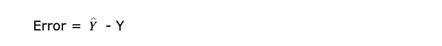
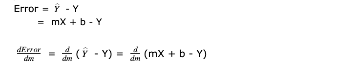
So, Error is the difference between the two, that is,

the predicted value – correct value

It relates to the idea of cost/loss function.

Let’s see what does cost/loss function does and why do we need it.

Concept of Cost / Loss Function

The Loss function computes the error for a single training example.

The Cost function is the average of the loss function for all the training examples.

Here, both the terms are used interchangeably.

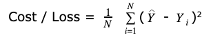
If you want to evaluate how your ML algorithm is performing, for a large data set what we do is take the sum of all the errors.

_{Image Source: Created by Author}

This is the total error for the particular model, being m and b values that describe that line.

Our goal is to minimize that loss. We want the lowest error. That means we want the lowest m and b values to get the lowest error.

So, the above cost function is equivalent to Y = f(x) = X²

If you graph Y = X² on the Cartesian Coordinate system, it will look as follows:

Suppose we are considering Q as the current data point. We have to find the minima which is at point O. Then there are 2 things that we need

1. Which direction to go (Direction of update)

2. How big step to take (Amount of update )

The way to find minima is by taking a derivative (also known as gradient).

The gradient of a curve at any point is given by the gradient of the tangent at that point.

Also, the gradient of a curve is different at each point on the curve.

See the above diagram carefully. Gradients are different at all the points P, Q, R, S, and O.

So the most common ways to look at derivatives are:

1. The Slope of the tangent line to the graph of the function

2. Rate of change of the function

Here the goal is to find a line that has the smallest error.

It means minimizing a function means actually finding the X value that produces the lowest Y.

So, this idea of being able to compute the slope(derivative) of this function tells us how to search and find the minima.

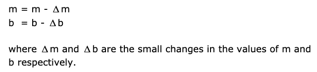
Parameters m and b with a slight change can be written as:

So, we want to know what is the way we can change the value of m in y = mx + b in order to make the error lesser. Hence, the next step is to find the m and b values with the lowest error. It can be done by finding the derivative (gradient) of this cost/loss function to know which way to move.

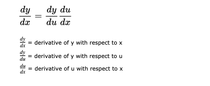
Here, we will be using the following 2 rules of calculus to find the derivative:

1. Power Rule:  
2. Chain Rule:

_{Image Source: Created by Author}

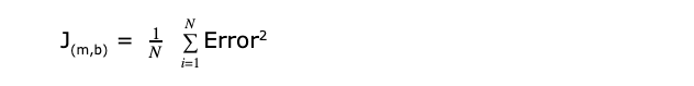
Let’s say J_(m,b) is the Cost / Loss function in m and b.

👁 loss function| Gradient descent algorithm

_{Image Source: Created by Author}

Let us assume that we are looking at one error at a time. So we will get rid of the summation sign.

J_(m,b) = Error²

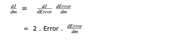
Differentiating J with respect to m and applying Power rule and Chain Rule

We are applying the chain rule because J is a function of Error and Error is a function of m and b.

_{Image Source: Created by Author}

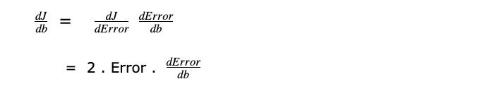
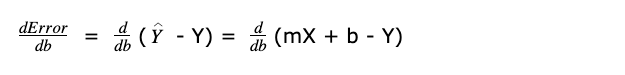
Similarly, differentiating J with respect to b

As discussed above,

X is input data, b is constant and Y is output.

Derivative of constant is Zero because constant does not change and derivative describes how something changes. Hence derivatives of b and Y are zero.

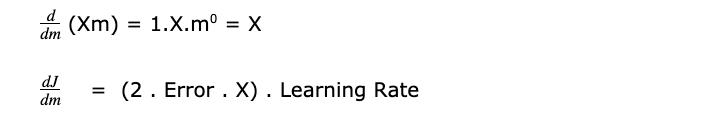
According to the power rule,

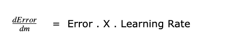
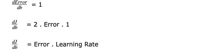
We can get rid of 2 as it just tells how big or small the learning rate is. So it’s not significant.

_{Image Source: Created by Author}

(Error . X) decides direction as slope/derivative contains the direction information.

Learning rate decides step size/amount of update.

Differentiating Error with respect to b

_{Image Source: Created by Author}

X is input data, m is constant and Y is output. As discussed earlier,

_{Image Source: Created by Author}

According to the update rule,

_{Image Source: Created by Author}

EndNote

The Gradient Descent Algorithm helps improve machine learning models by reducing errors. It works by adjusting the model’s parameters step by step, following the slope of a cost or loss function, which measures how far the model’s predictions are from the actual values. Starting with a basic model, Gradient Descent refines it by continuously lowering this error. The key idea is to minimize the cost function, making the model’s predictions more accurate over time. This method is essential for building better-performing machine learning models.

Login to continue reading and enjoy expert-curated content.

Free Courses

Become an Author

Share insights, grow your voice, and inspire the data community.

• Reach a Global Audience
• Share Your Expertise with the World
• Build Your Brand & Audience

• Join a Thriving AI Community
• Level Up Your AI Game
• Expand Your Influence in Genrative AI

👁 imag