 |
VOOZH | about |
|
VOOZH | about |
The Friedman Test is a non-parametric statistical test used to detect differences in treatments across multiple test attempts. It is often used when the data is in the form of rankings or ordinal data, and when you have more than two related groups or repeated measures. The Friedman test is the non-parametric alternative to the repeated measures ANOVA and is useful when the assumptions of normality and homogeneity of variances are not met
The Friedman test is used to compare three or more related groups or repeated measures. It analyzes the ranks of the data rather than the raw values, which makes it ideal for non-parametric data.
Null Hypothesis: There is no significant difference between the given conditions of measurement OR the probability distributions for all the conditions are the same. (Medians are same)
Alternate Hypothesis: At least 2 of them differ from each other.
H0 : M1 = M2 = M3 = ..... Mk ; M= Median
H1 : At least two of them show significant difference.
To calculate the test statistic for the Friedman test
Where:
You can make the decision on the basis of the below-mentioned rules-
If the null hypothesis is rejected in the Friedman test, post hoc analysis helps identify which specific pairs of experimental conditions differ. This can be done using tests like the Wilcoxon signed-rank test or Conover's test.
For the Wilcoxon signed-rank test, results for all pairs can be obtained, but a Bonferroni correction is necessary. This correction adjusts the significance level to (Given significance level / total number of pairs) to control for Type I errors.
Let us take an example to understand how to perform this test.
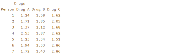
Example: random people were given 3 different drugs and for each person, the reaction time corresponding to the drugs were noted. Test the claim at the 5% significance level that all the 3 drugs have the same probability distribution.
| Drug A | Drug B | Drug C | |
|---|---|---|---|
| 1 | 1.24 | 1.50 | 1.62 |
| 2 | 1.71 | 1.85 | 2.05 |
| 3 | 1.37 | 2.12 | 1.68 |
| 4 | 2.53 | 1.87 | 2.62 |
| 5 | 1.23 | 1.34 | 1.51 |
| 6 | 1.94 | 2.33 | 2.86 |
| 7 | 1.72 | 1.43 | 2.86 |
Step 1: Define NULL and Alternate Hypothesis
Step 2: State Alpha (Level of Significance)
Step 3: Calculate Degrees of Freedom
Step 4: Find out the Critical Chi-Square Value.
Step 5: State Decision Rule
You can check for any of the two rules:
Step 6: Assign Ranks for the drugs corresponding to each person and find the sum.
| Ranks | |||
|---|---|---|---|
| Drug A | Drug B | Drug C | |
| 1 | 1 | 2 | 3 |
| 2 | 1 | 2 | 3 |
| 3 | 1 | 3 | 2 |
| 4 | 2 | 1 | 3 |
| 5 | 1 | 2 | 3 |
| 6 | 1 | 2 | 3 |
| 7 | 2 | 1 | 3 |
| ∑ = 9 | ∑ = 13 | ∑ = 20 | |
Note: If in the same row 2 or more columns have the same value then the rank assigned to them is the average of the ranks they get. For example: If a row has 2 columns with value x and the ranks which they get are 4 and 5. Then both the columns will be assigned with a rank of (4+5)/2 which is 4.5.
Step 7: Calculate Test Statistic
The Friedman test statistic formula is:
Where:
= 8.857
Step 8: State Results
Since FR is greater than 5.991 , We reject the Null Hypothesis.
Step 9: State Conclusion
Here,
Total number of pairs can be 3 (Drug A - Drug B , Drug B - Drug C , Drug A - Drug C).
The new level of significance to be considered for each pair will be 0.05/3 = 0.0166.
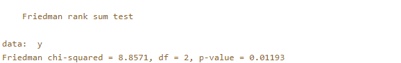
Output:
👁 ImageOutput:
👁 ImageAs the p-value is less than the significance level (5%) it can be concluded that there are significant differences in the probability distribution.