Google Sheets NOT Function: A Complete Guide with Examples

The NOT function in Google Sheets is a powerful logical tool used to reverse the result of a given condition. By inverting TRUE to FALSE and vice versa, the NOT function is essential for building more complex formulas and logical expressions. It helps refine your calculations, making it easier to create dynamic and flexible spreadsheets. Whether you're combining it with IF, or OR functions, the NOT function simplifies decision-making processes within your data, offering more control and precision over your results.

1. NOT formula in Google Sheets

The NOT function in Google Sheets is a logical function that reverses the logical value of its argument. If the argument is TRUE, it returns FALSE; if the argument is FALSE, it returns TRUE. This function is often used to invert conditions or to apply additional logic in formulas.

How It Works:

• The NOT function takes a single logical condition as its argument.
• If the condition evaluates to TRUE, the NOT function will return FALSE.
• If the condition evaluates to FALSE, the NOT function will return TRUE.

Google Sheets NOT Function Syntax:

=NOT(logical)

• logical: This is the condition you want to evaluate. It can be a reference to a cell, a logical expression, or another function that returns a logical value.

2. How to Use the NOT Function in Google Sheets

The Google Sheets NOT formula is a simple yet powerful tool to reverse logical values. Here’s how to use it effectively with examples of the NOT function:

Step 1: Select the Cell for the Formula

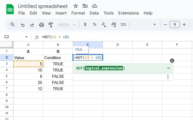
Click on the cell where you want to display the result of the formula.

Step 2: Enter the NOT Formula

In the selected cell, type the formula:

=NOT(A3 > 10)

This formula will return FALSE if the condition A1 > 10 is true, and TRUE otherwise.

Step 3: Press Enter to Apply the Formula

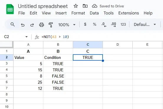
Hit Enter to apply the formula. The result will display TRUE or FALSE based on the logical condition.

3. Combining Not with IF, and OR functions in Google Sheets

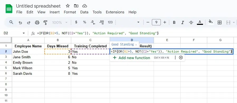
The NOT function in Google Sheets is a versatile logical operator that reverses any condition, making it perfect for refining complex formulas. It works seamlessly with functions like IF, OR, and ISBLANK to create smarter, condition-based calculations. Here we will use NOT function with IF and OR making it complex to solve other problems.

Step 1: Set Up the Data and Select a Cell

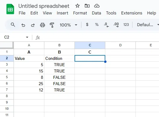
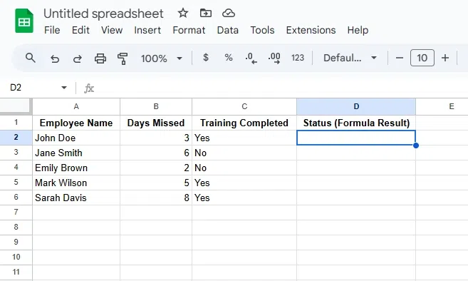
Create a table with columns for employee names, days missed, and training status. For instance:

• Column A: Employee Name
• Column B: Days Missed
• Column C: Training Completed (Yes/No).

Step 2: Write the Formula

In a new column (e.g., Column D), enter the following formula:

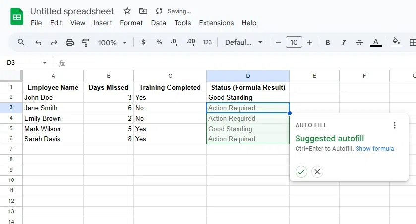
=IF(OR(B2>5, NOT(C2="Yes")), "Action Required", "Good Standing")

• B2>5 checks if the employee missed more than 5 days.
• NOT(C2="Yes") checks if training is not completed.
• OR ensures that if either condition is true, the action is triggered.
• IF determines the result based on the condition.

Step 3: Apply the Formula Across Rows

Drag the formula down the column to evaluate all employees.

Step 4: Interpret the Results

• "Action Required" will appear if the employee meets either condition (missed more than 5 days OR has not completed training).
• "Good Standing" will appear if neither condition is true.

With the Google Sheets NOT formula, you can handle data logic efficiently and customize spreadsheet workflows.

Also Read:

• Google Sheets IF Function
• How to use AND in Google Sheets: A Complete Guide
• OR Logical Function in Google Sheets