 |
VOOZH | about |
|
VOOZH | about |
A function is a built-in formula in Excel that performs calculations using specified values in a set order. Excel offers many common functions to quickly compute the sum, average, count, maximum, and minimum values of a cell range. To use functions effectively, you need to understand their components and how to create arguments for calculating values and cell references.
Table of Content
A Google Sheets function is a calculating tool available in the spreadsheet program. Using a particular function, you may sort data and see how it relates to other data points as you enter it. The intricacy of these functions varies. Some solve fundamental mathematical problems, while others aid in comprehending more intricate data.
Just like with formulas, the order in which you enter a function in a cell matters. Each function has a specific syntax that must be followed to work correctly. To create a function formula, start with an equals sign (=), followed by the function name (like AVERAGE for finding an average), and then the argument. The argument includes the information or cell range you want to calculate.
Create a new spreadsheet or open an existing one.
Click on the cell where you want to use the function.
Start with an equal sign (=), followed by the function name.
Example: =SUM(A1:A10)
Here are 14 Google Sheets functions you can use to make managing data easier:
One of Google Sheets' most fundamental operations is the SUM function. The SUM function allows you to add several cells at once.
On the right-hand side, you will see dots, and tap on it. Scroll it down, and you will see Google Sheets. Please open it and choose a blank page.
Click on an empty cell where you want the total to show up.
Type =SUM(B2:B7).
Press Enter, and you will get the SUM.
Example of SUM Function:
=SUM(A5:A10)
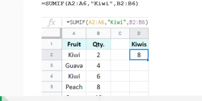
The SUMIF function lets you determine the total number of cells that satisfy specific requirements.
Select the cells with the data and the enter the formula =SUMIF(A:A,"Text",B:B).
Click and drag all the numbers across the cells that you want to add up in (). Click Enter.
Example of SUMIF function:
=SUMIF(A:A,"Text",B:B)
Use the COUNT function to determine how many cells in a range contain a value. The steps below are provided for your convenience.
In that cell, type =COUNT( (equal sign, then COUNT followed by an opening parenthesis).
Click and drag across all the cells containing the data you want to count. It can be text, numbers, or even dates!
Example of COUNT function:
=COUNT(D:D)
You may input the current date into a spreadsheet cell using the TODAY function.
In that cell, type =TODAY() (equal sign followed by TODAY and parentheses). Click Enter.
Examples of TODAY function:
=TODAY() or =TODAY()+5
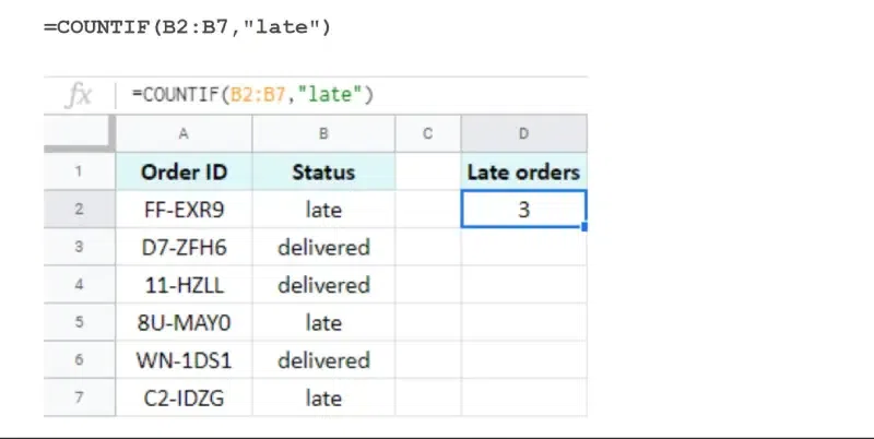
If specific criteria are met, the COUNTIF function lets you count the number of cells in a range that contain a value.
Type =COUNTIF( (equal sign, then COUNTIF followed by an opening parenthesis). Click and drag across all the cells you want to consider (like A1:A10) and type in (). Click Enter.
Example of COUNTIF function:
=COUNTIF(A:A,"Text")
The AVERAGE function determines the AVERAGE function determines the data. You can enter either or calculate an average of calculate in a specific column or row.
In that cell, type =AVERAGE (equal sign, then AVERAGE followed by an opening parenthesis). Click Enter.
Example of AVERAGE function:
=AVERAGE(A:A)
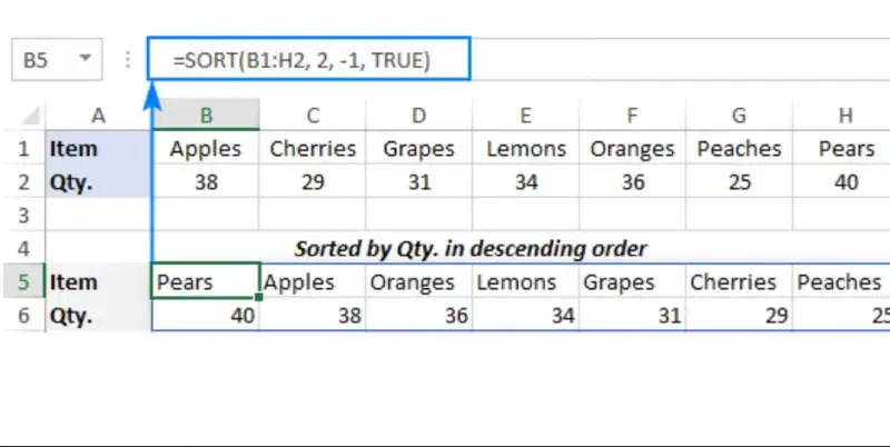
Cells containing numerical data can be sorted using the SORT algorithm from lowest to highest value.
Type =SORT( (equal sign followed by SORT and an opening parenthesis). Click and drag across all the cells you want to sort. Click Enter.
Example of SORT function :
=SORT(A:A,1,TRUE)
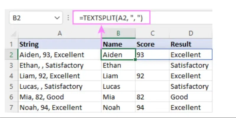
Using the SPLIT function, you can split text from a single cell into numerous cells.
In cell B1, type =SPLIT( (equal sign, then SPLIT followed by an opening parenthesis). Choose Your Text to Split.Tell it Where to Split. Click Enter.
Example of SPLIT function:
=SPLIT(A8,"text")
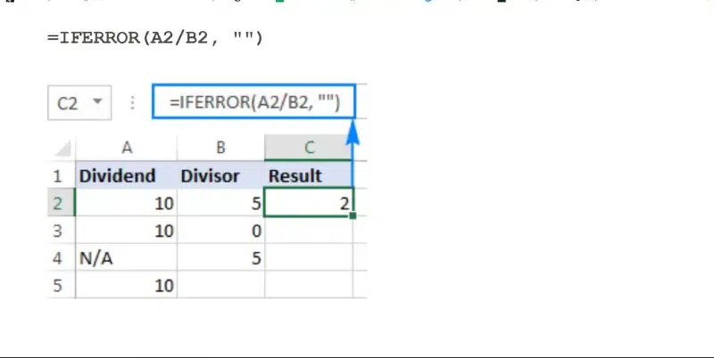
If a function produces an error in a specific cell (or set of cells), you may use the IFERROR function to find the value for that cell.
In that cell, type =IFERROR( (equal sign, then IFERROR followed by an opening parenthesis).Inside the parenthesis, type the function you're hoping will work.
If you want to see a message like "Error" or "Data Missing" when the function runs into trouble, type that message in quotes after the comma (,) and press Enter.
Example of IFERROR Function:
=IFERROR(A:A,"AnyText")
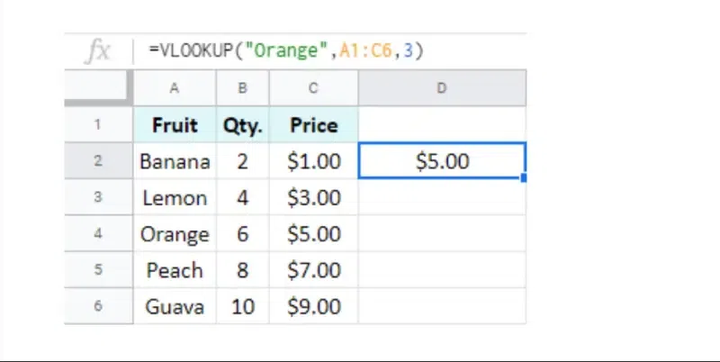
You may search for particular data inside the spreadsheet using the vertical lookup, or VLOOKUP, feature.
Type =VLOOKUP(. Click the cell with your search code.
Select your entire table of codes and details. Select the Column. And click Enter.
Example of VLOOKUP Function:
=VLOOKUP(B5, 'Sheet1'!B: C,2, FALSE)
With the help of this thorough guide, you can finally master Google Sheets! We'll reveal the secrets of everyday functions like SUM, AVERAGE, and COUNT, which will simplify data processing. We don't stop there, though! We'll go further, teaching you how to adjust functions and solve problems in the real world. You'll turn your spreadsheets into dynamic, problem-solving powerhouses capable of handling anything from budget management to survey analysis. Prepare to unlock your data's full potential.
Are spreadsheets limited to basic math?
No, Google Sheets has functions beyond addition and subtraction. You can use them to find specific information (VLOOKUP) or make decisions (IF).
How to use VLOOKUP in Google Sheets
- Organize your data. Enter your data into a spreadsheet or locate an existing table.
- Select an output cell.
- Enter the VLOOKUP function.
- Enter the search_key.
- Set the value range.
- Set the index column.
- Determine is_sorted value.
- Execute the function.