Comprehensive guide for Data Exploration in SAS (using Data step and Proc SQL)

9 min read

Introduction

I would like to extend my sincere gratitude to our readers for their overwhelming response on my previous articles on data exploration. These articles featured: variable identification, Univariate and Bivariate analysis, Missing and Outlier identification and treatment and feature engineering.

In this guide, I will take a step ahead and show all these steps to explore data sets practically in SAS. I will also perform some exercises that will help you understand the concept better. You can look at this article as practical implementation of my previous articles (in SAS).

I am hoping that this guide can act as a ready reference for our followers trying to navigate SAS on their own. Let’s get down to work!

👁 Comprehensive guide for Data Exploration in SAS (using Data step and Proc SQL)

Contents:

Since this is an exhaustive guide, it is a good idea to list down all the things I’ll cover:

1. 1. How to load data file(s) into SAS Data set?

   2. How to convert a variable to different data type?

   3. How to transpose a Data set?

   4. How to sort Data set in SAS?

   5. How to create plots (Histogram, Scatter, Box Plot) in SAS?

   6. How to generate frequency tables in SAS?

   7. How to do sampling of Data set in SAS?

   8. How to remove duplicate values of a variable?

   9. How to group variables in SAS to calculate count, average, sum?

   10. How to recognize missing values and outliers?

1. How to impute missing values and outliers?

2. How to drop and rename variables in a data set?

3. How to merge / join data set effectively?

Part 1: How to load data file(s) into SAS Data set?

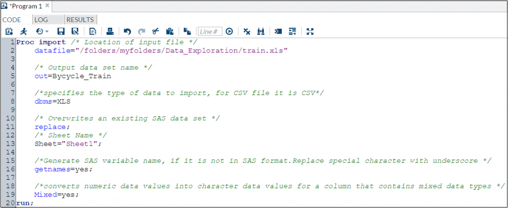
The sources of input data sets can be in various formats (.XLS, .TXT, .CSV) and sources like databases. In SAS, we can use multiple methods to load data from these sources. Let’s look at the commands to load data from each dataset type mentioned above:

1. Proc Import
2. Data Step

Importing XLS/ CSV file using PROC Import:

👁 Proc Import, SAS, Excel

Notes:

• Both .xls and .xlsx files can be imported.
• To import a .xlsx file, simply change xls to xlsx in both the datafile and the dbms line.
• For importing CSV file, use CSV for dbms line.

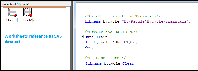
We can also create a library from excel files using Libname statement (Each worksheet in the Excel workbook is treated as a SAS data set. Worksheet name appears with a dollar sign at the end of the name).

👁 Libname, Libref, SAS

If SAS has a libref assigned to an Excel workbook, the workbook cannot be opened in Excel. To disassociate a libref, use a LIBNAME statement and specify the libref and the CLEAR option.

Importing raw text file (Txt) using PROC Import:

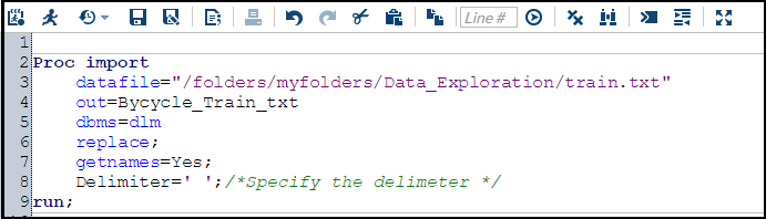
If your data file is a simple text file, you can use following commands:

👁 Proc Import, txt, SAS

It is assumed that the first row of the data set contains column names. If first row is not the column name, then we would change getnames=yes to getnames=no. After that, names of the columns would get stored as VAR1 to VARn.

Importing using Data step:

You can also make use of Data Step to import data from csv or text file.

Syntax:

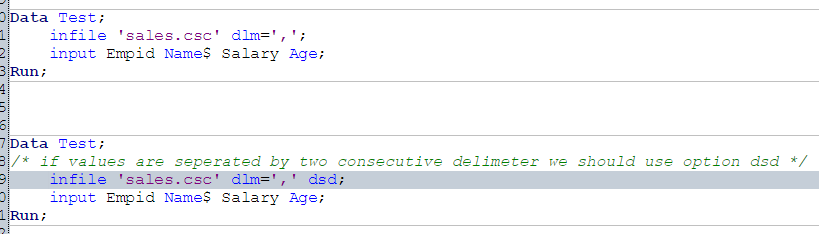
Data output_set;
 INFILE 'raw_data_file_name';
 Input specifications;
 <additional statements>;
 Run;

Example: Import data from a csv file using data step, assuming values are separated by comma(,).

👁 Input

Above, we looked at multiple methods to load data set in SAS. To load data set from databases like ORACLE, SQL SERVER and others, we would require authorization from both SAS Admin or Database admin.

To explore this in detail, you can refer to links below:

• Resource 1
• Resource 2
• Resource 3

Part 2: How to convert a variable to different data type?

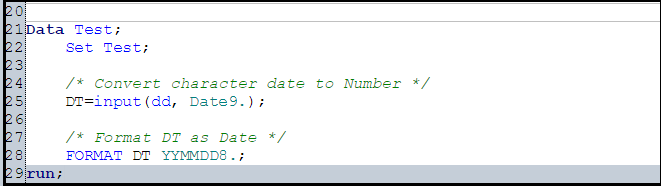
We can convert character to numeric and numeric to character and also change the format of variable like number to date, date to number, number to currency format etc. Let’s look at some of the commands to perform these conversions:

1. Convert numeric variables to Character variables and vice versa

To perform this, we will use INPUT function. It takes two arguments: the name of a character variable and a SAS informat or user-defined informat to read the data.

Syntax:  

INPUT (Source, Informat)

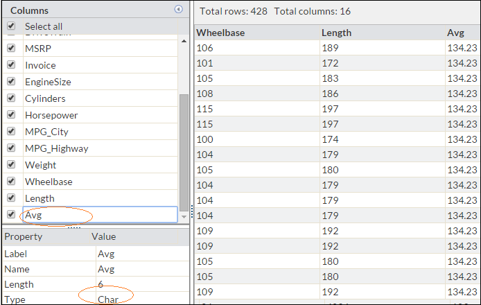
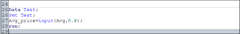
In snapshot below, you can see that variable Avg is in character format. Now to convert it into number, we’ll use Input function.

👁 INPUT, Put, SAS, Conversion

See below codes:

👁 Input, SAS

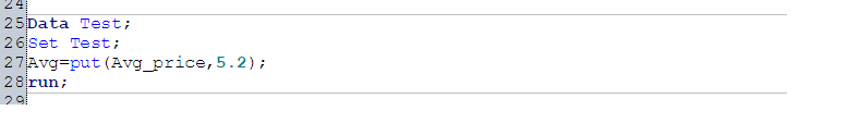
Similarly, if we want to convert a numeric variable to character, it can be done using PUT function.

Syntax:

Put(Source, Format)

👁 Put, SAS

       2. Convert character date to Date

👁 SAS, Character Date to Number

For more details on Input and Put function, you can refer below links:

• Resource 1
• Resource 2

Part 3: How to transpose a Data set?

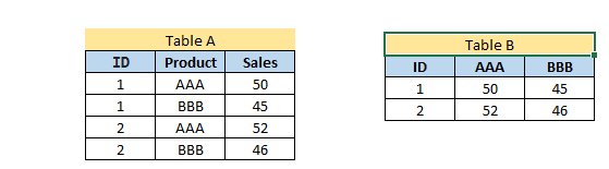
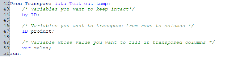
Let us say, we want to transpose Table A into Table B on variable Product. This task can be accomplished in SAS using PROC Transpose:

👁 Transpose, SAS

👁 Transpose, SAS

For more detail on PROC Transpose, refer  below link:

• Resource 1
• Resource 2

Part 4: How to sort Data set in SAS?

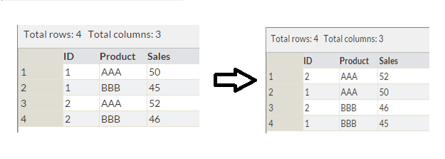
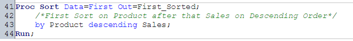
Sorting of data can be done using procedure PROC SORT. It can be based on multiple variables and ascending or descending both order.

Syntax:

PROC SORT Data = Input_data_set <Out = Output_data_set>;
 By <Descending> Variable_1 <Descending Variable_2 ....;
 Run;

👁 Sort, SAS
Above, we have a table with variables ID, Product and Sales. Now, we want to sort it by Product and Sales (in descending order) as shown in table 2. This can be done using Proc Sort as shown below.

👁 SORT, PROC SORT, SAS

Part 5: How to create plots (Histogram, Scatter, Box Plot) in SAS?

👁 Plot, Histogram, Box Plot, Scatter Plot, Proc SGPLOT, Proc GPLOT, Proc Univariate

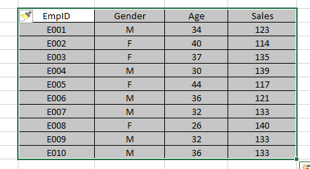
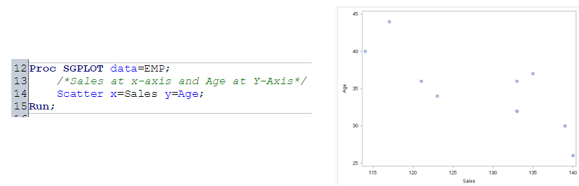
Let’s understand plots using the example shown above. We have employee details with their EmpID, Gender, Age and Sales Detail. We want to understand:

• The distribution of age
• Relation between age and sales; and
• If sales are normally distributed or not?

These tasks can be accomplished by using Scatter, Box and Histogram representation.

Histogram:

Now to understand the distribution and check whether the data is distributed normally or not, we will plot a Histogram. In SAS, histograms can be produced using PROC UNIVARIATE, PROC CHART, or PROC GCHART. Here we will use PROC UNIVARIATE with the HISTOGRAM statement.

👁 Histogram, Proc SGPLOT

Scatter plot:

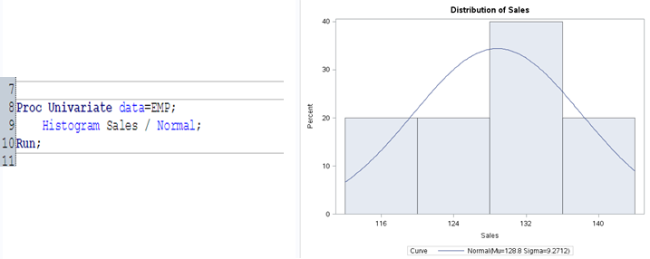
It is used to find the relation b/w two continuous variables.  Here we will use PROC SGPLOT to plot scatter graph.

👁 Scatter, PROC SGPLOT, SAS

Box-plot:

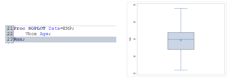
Box-Plot is used to understand the distribution of continuous variables. This is also known as five number summary plot of Min, First Quartile, Median, Third Quartile and Max. We will again use PROC SGPLOT to display the Box-plot.

👁 Box Plot, SAS, Proc SGPLOT
For more details on PROC Univariate and PROC SGPLOT, you can refer below links:

• Resource 1
• Resource 2
• Resource 3

Part 6: How to generate frequency tables in SAS?

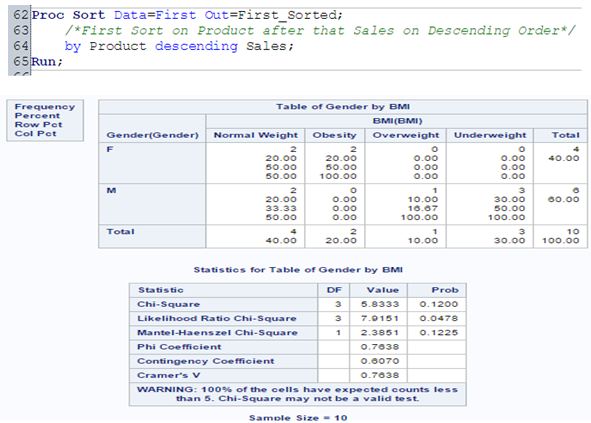
Frequency Tables can be used to understand the distribution of a categorical variable or n categorical variables using frequency tables. We will use PROC FREQ procedure to perform this.

PROC FREQ is capable of producing statistical test and other statistical measures in order to analyze categorical data based on the cell frequencies in 2-way or higher tables.

I have added another variable BMI to above mentioned employee table. Now, to understand the distribution between GENDER and BMI, I will use PROC FREQ procedure with CHISQ statistical test.

👁 Frequency Table, Proc Freq, SAS


For more detail on PROC FREQ, you can refer below link:

• Resource

Part 7: How to do sampling of Data set in SAS?

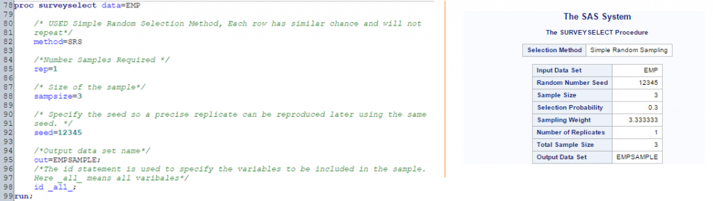
To select an unbiased sample from a larger data set in SAS, we use procedure PROC SURVEYSELECT. Here we will go with PROC SURVEYSELCT.

Let’s say, from EMP table, I want to select random sample of 3 employee.

👁 Sample, Proc Surveyselect, SAS

Part 8: How to remove duplicate values of a variable?

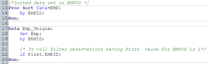
Often, we encounter duplicate observations. To tackle this, SAS has multiple options like FIRST., LAST., NODUPKEY with PROC SORT ,PROC SQL and others. Let’s understand these options one by one:

Method 1. Using First. or Last.

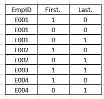
To use First. or Last. option, data set must be sorted by variable(s) on which we want to identify the unique records. First. and Last. automatic variables created by SAS when using by-group processing. It has value of 0 and 1.

• If it is first observation of duplicate values of ‘by variable’ then value of variable First. would be 1 else 0
• For Last variable, it would be 1 if last observation of duplicate values of ‘by variable’ else 0.

👁 first., Last., Proc Sort, SAS

Above, you can see that how value of First. and last. is populated. Now, let’s see how can we use these two values to identify unique records.

👁 First., Last., SAS

Above, we have used first. to filter first observation and to filter last observation, we can use Last. 

Method 2. NODUPKEY with Proc SORT

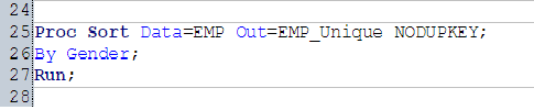
We can use NODUPKEY option with Proc Sort to remove duplicate values.

👁 NODUPKEY, PROC SORT, SAS

Method 3. Binning Numerical Variable

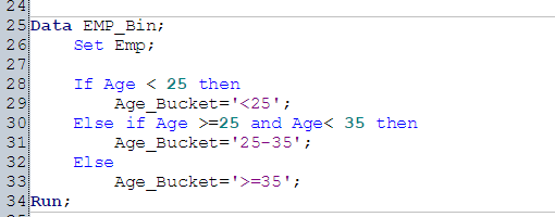
We can use conditional statements and logical operators to bin numerical variables. In Emp data set, we have variable Age. Here we will bin variable Age as <25, >=25 and <35, >=35.

👁 Binning, SAS

Part 9: How to group variables in SAS to calculate count, average, sum?

To understand the count, average and sum of variable, I would suggest you to use PROC SQL with group by. There are other methods also like Proc FREQ and PROC Means to perform.

Let’s look at the syntax of these Procedures:

PROC SQL:

PROC SQL;
 Create table <Output Data set> as
 Select Count(Var1), Sum(Var2), Average(Var2) from <Input Data set> group by Var4, Var5...;
 Quit;

PROC Means:

PROC MEANS Data=<Input Data Set>;
 VAR Varibales(s);
 Class Classification_Varibale(s);
 Run;

Part 10: How to recognize missing values and outliers?

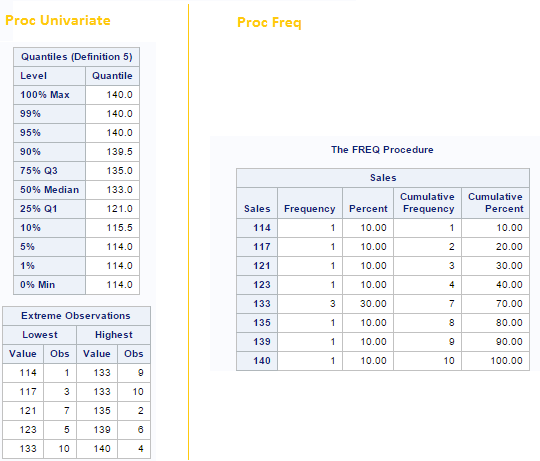
To identify outliers in a variable, we can go with Proc Univariate procedure and use PROC FREQ to identify missing values. Let’s look at the output below to understand these two procedures:

👁 PROC Univariate, Proc Freq, SAS

Above, you can see that PROC Univariate as shown top and bottom 5 values whereas PROC FREQ shows the distribution of unique values of variable.

Part 11: How to impute missing values and outliers?

There are various imputation methods available for missing and outlier imputation. You can refer these articles for methods to detect Outlier and Missing values. Imputation methods for both missing and outlier values are almost similar. Here we will discuss general case imputation methods to replace missing values. Let’s do it using an example:

Let’s say we have an employee data set comprising of multiple variables like Empid, Name, Gender, Sales, Age, Region, Product and other. Here, we want to predict the sales of employee. But, one of the concern is variable Age has missing values and variable Age appeared as significant variable.

Now to deal with this missing values, I have written below SAS statements:

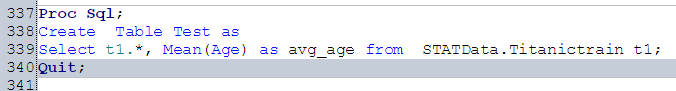
Identify Values to Impute Using General Case Method (Average of Age):

👁 First

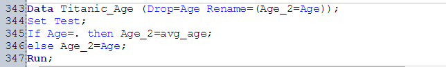
Imputation Using Data Step

👁 Second

Above, you have seen one of the methods to deal with it. You can also use multiple methods using SAS statements. I would suggest you to practice all the discussed method in my previous post on missing values and outliers.

Part 12: How to drop and rename variables in a data set?

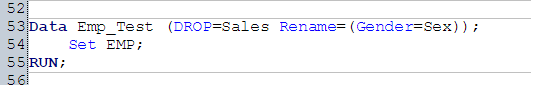
Let’s say, during data exploration stage, we want to exclude variables those are not required in the data modelling exercise or want to rename few variables also. These two operations can be performed using DROP and RENAME options using DATA STEP.

Let’s say, we want to drop variable AGE and rename variable Gender as Sex. This can be performed using below statement.

👁 DROP_Rename_Varibales

Part 13: How to merge / join data set effectively?

Merging / Joining can be of various types. It depends on the business requirement and relationship between data sets. In SAS, we can perform this in various ways using DATA STEP, PROC SQL and PROC Format. Now, question is, which is the most appropriate method to perform merging and joining?

You can refer on of my post on this topic for detailed info. here: Introduction to Merging.

End Notes:

In this guide, we looked at the SAS statements for various steps in data exploration and munging like loading of data, converting data type, transposing tables, sorting, plotting, removing duplicate values, binning, grouping, identifying missing & outlier values, dropping & renaming variables, merging & joining tables and imputing values for missing and outlier values. We also looked at the basic SAS statement to perform this and have given links to look at more advance methods.

In one of the next article, I will reveal the codes to perform these steps in Python. Stay Tuned!

Did you find the article useful? Do let us know your thoughts about this guide through comments below.

If you like what you just read & want to continue your analytics learning, subscribe to our emails, follow us on twitter or like our facebook page.

Login to continue reading and enjoy expert-curated content.

Free Courses

Become an Author

Share insights, grow your voice, and inspire the data community.

• Reach a Global Audience
• Share Your Expertise with the World
• Build Your Brand & Audience

• Join a Thriving AI Community
• Level Up Your AI Game
• Expand Your Influence in Genrative AI

👁 imag