Introduction to Artificial Neural Network with Implementation

Overview

This article will support data scientists in furthering their studies on artificial neural networks so that they can develop applications for professional use.

We introduce the concept of ANN, from the Perceptron device, we conceptualize input neurons, functions, and activation functions for the calculation of the output neuron. The concept of the descent gradient is very important to the data scientist.

We will present two implementations of Neural Networks:

i) Neural Network with Orange Data Science using visual programming, using components on a canvas.

ii) Deep Learning with the Tensor Flow Framework, with the Python programming language.

Before, we dig in deep into the article. Would you like to read the introduction to Artificial Neural Networks?

Table of Contents

1. 1. Introduction
2. 2. Neural Network with Orange
3. 3. Deep Learning with TensorFlow
4. 4 Other Neural Network Architectures
5. 5 Conclusions
6. 6 References

Introduction

In this section, we will address the theoretical themes of artificial neural networks

• Perceptron,
• Sum Function,
• Activation Function,
• Multilayer Perceptron
• Error Calculation,
• Gradient Descent,
• Backpropagation

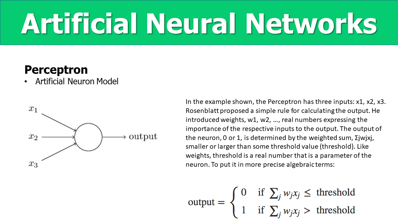
1.1 Perceptron

Perceptron is a model for understanding a single-layer ANN. Perceptron device makes decisions by proving the evidence of the input variables x1,x2,…xn.

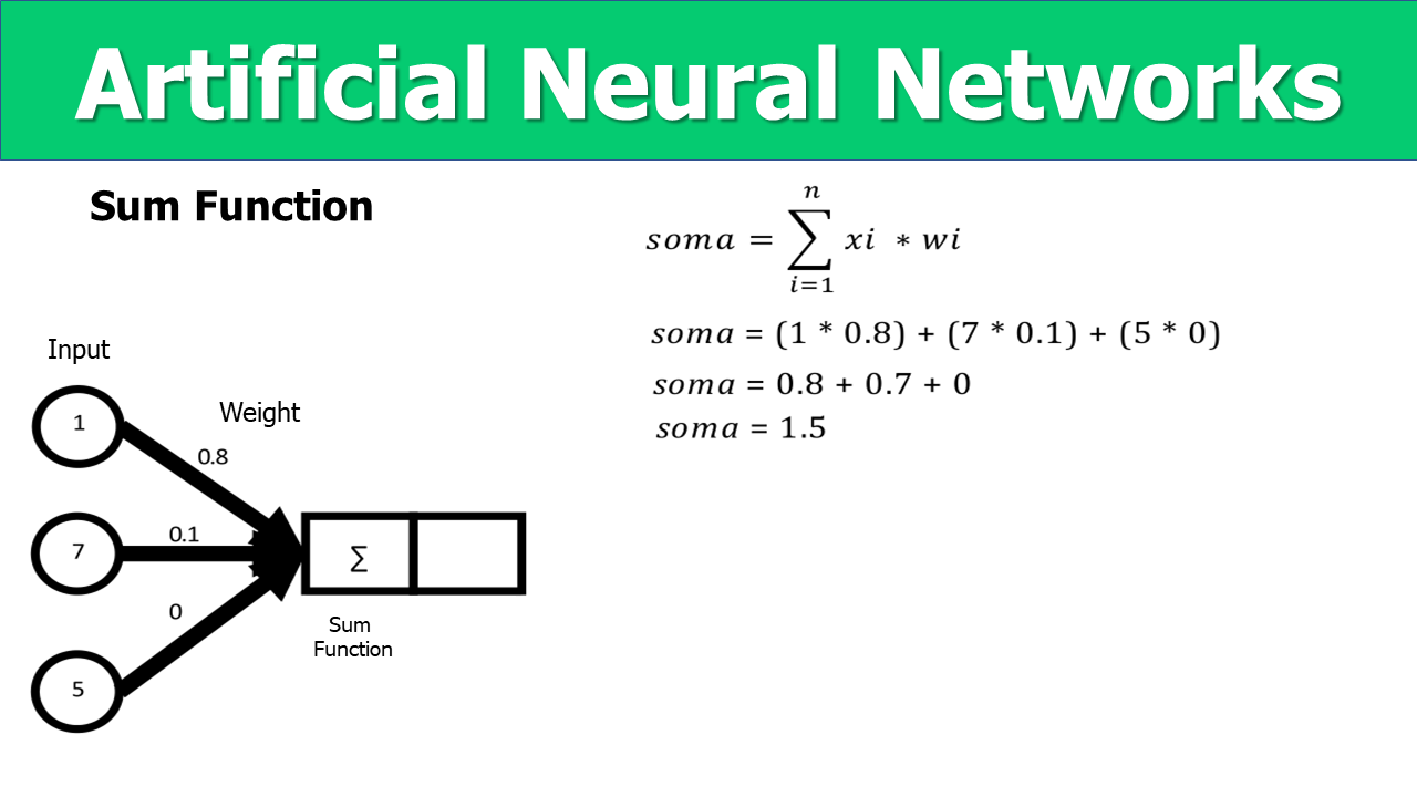
1.2 Sum Function

We have the inputs to a neuron and have an associated weight, later we have the sum function and the activation function, a step function.

https://github.com/DataScience-2021/Analytics-Vidhya/blob/main/_Neural_Networks/Neural_Networks%20-%20Projeto/Slide4.PNG

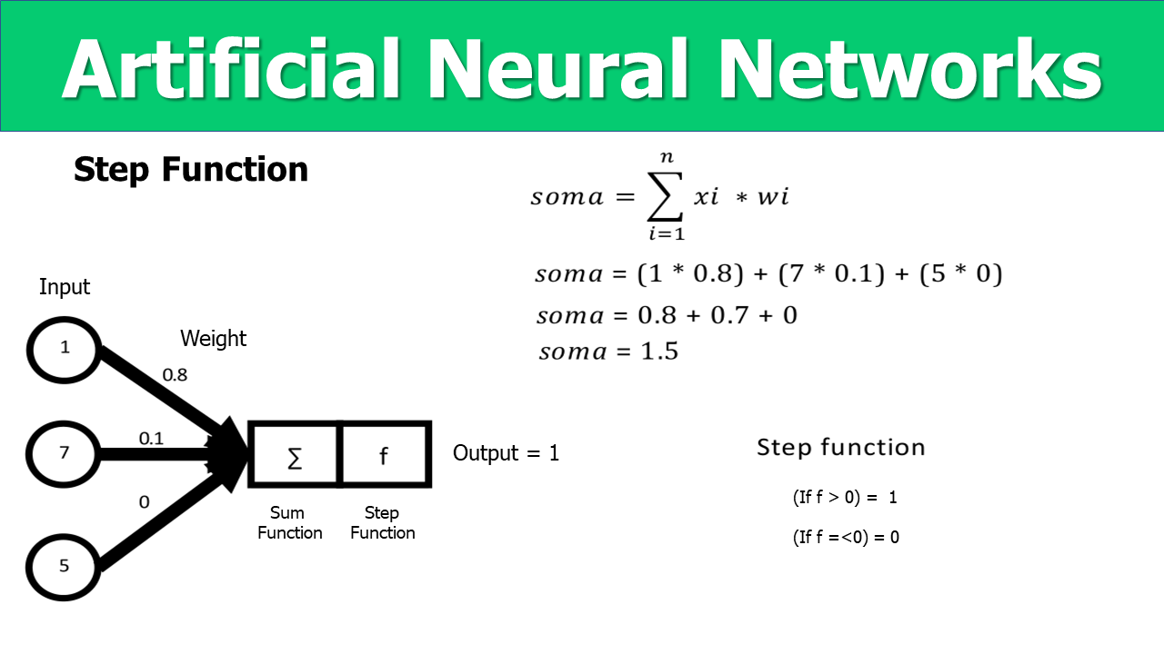
1.3 Activation Function

The activation function is responsible for processing the output of the ANN, in this article, we use the step function, which outputs the value 1 if the result of the sum function is > 0, and outputs the value 0 for results many different.

https://github.com/DataScience-2021/Analytics-Vidhya/blob/main/_Neural_Networks/Neural_Networks%20-%20Projeto/Slide5.PNG

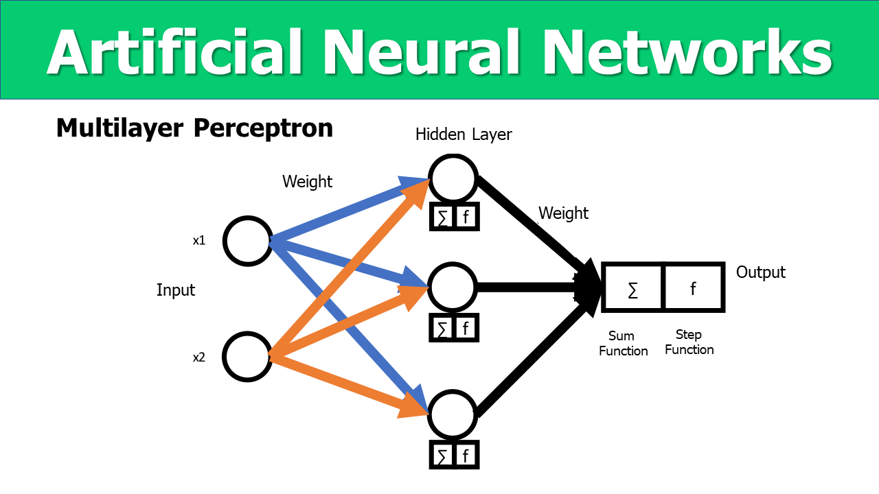
1.4 Multilayer Perceptron

Multilayer networks have more than one hidden, which is one of the characteristics of Deep Learning. In conjunction with activation function, sigmoid function.

We visualized below the processing of a multilayer ANN, which from the input values in the ANN, these values are multiplied by their respective weights, and the output is the result of processing the weights with the activation function.

https://github.com/DataScience-2021/Analytics-Vidhya/blob/main/_Neural_Networks/Neural_Networks%20-%20Projeto/Slide6.PNG

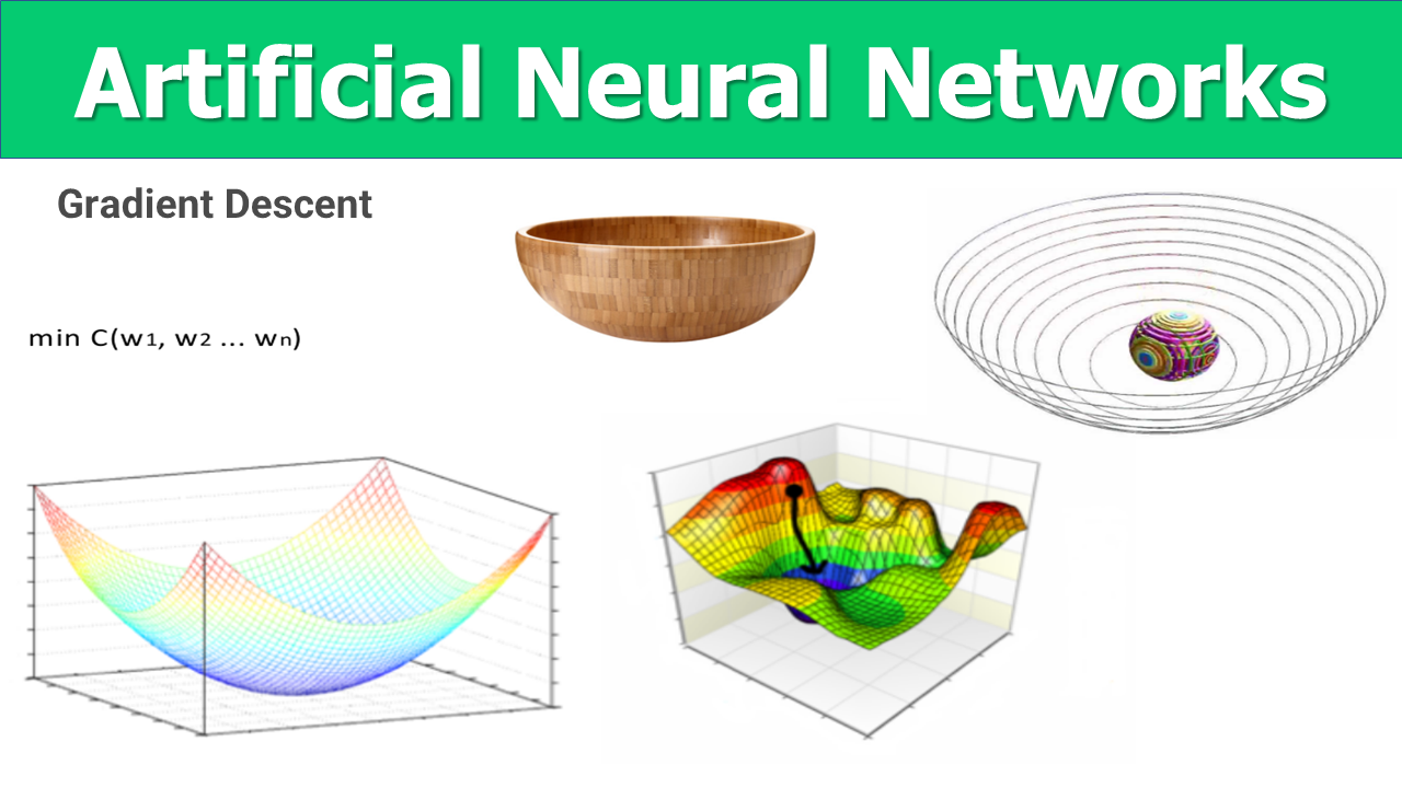
1.5 Gradient Descent

The Descending Gradient Model is made for the Data Scientist has to master the applied mathematical model, that the data entry starts at the top of the curve in 3D where the error is big, and in which it challenges us to find the weights. , that we can descend the gradient until we reach the curve in 3D, where the error is small.

The gradient’s descent, where it starts at the top with the high error until reaching the bottom with low error. For the run of this model, I apply the calculation of Partial Derivatives, which move to the gradient direction, to reduce the error.

https://github.com/DataScience-2021/Analytics-Vidhya/blob/main/_Neural_Networks/Neural_Networks%20-%20Projeto/Slide7.PNG

Objectives of Descending Gradient Calculation:

• Find the combination of weights so that the error can be inferior alternatives
• The Gradient is calculated to know how much to calculate weights

Stochastic:

Artificial Neural Networks with Orange

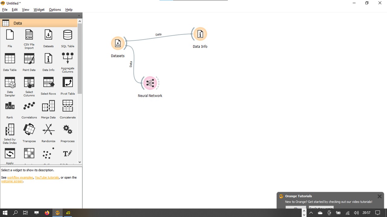
First, we select the ANN Object on Orange’s canvas, with a database to the object.

👁 Neural Network with Orange

https://orangedatamining.com/

In this section we will work with neural networks using the Orange tool, now it’s very similar to the other algorithms we’ve already used we’ll just select another algorithm that will be this Neural Network object.

👁 Neural Network with Orange 2

👁 Neural Network with Orange 3

This dataset is called Adult which just to recap We have data referring to the census. Out objectives is through all these attributes with age. Whether a person earns more than $50,000 a year or less than $50,000 a year.

And we are going to do a pre-processing on this data because when we work with neural networks we must normalize these data because note that this attribute is both a calculation performed by the census when this attribute and age are in very different scales and the algorithm in which it does distance calculations.

When you work with neural networks you must do this normalization. Otherwise, you will need to run the neural network more times, or else the results will not be that good.

So what we’re going to do is pull the preprocessing.

Here we have already defined the selection of characteristics, we are going to delete and we are going to choose the lines that have missing values ​​and we are also going to add or normalize the editors using standardization.

Demo ANN with Orange

For example, if it gets 10 it returns leaves and gets 15 and returns 15 and gets 30 if it gets a negative value for example minus 1 it changes to 0 if it gets minus 10 it changes to 0 if it gets minus 50 it changes to zero.

So this idea of ​​this function and we have the solver which is today the initiator, for example, a and the stochastic which includes indecent.

This is another one is the traditional gradient descent and Adam is the stochastic gradient decision. This is even the best user that is most used about the total number of repetitions.

Deep Learning with TensorFlow

!pip3 install seaborn

tf.__version__

dataset.head()

dataset.tail()

laranja_camisa_bartazul_calcao_bartazul_sapato_bartmarrom_boca_homerazul_calca_homercinza_sapato_homerclasse2880.00.00.00.0000006.4854120.093921Homer2890.00.00.00.0000000.0000000.042194Homer2900.00.00.00.0000004.2636290.076761Homer2910.00.00.00.0000001.4291330.017013Homer2920.00.00.013.7442480.8539020.063546Homer

sns.countplot(x = 'classe', data=dataset)

👁 Image

sns.heatmap(dataset.corr(), annot=True)

👁 Image

dataset.shape

(293, 7)

array([[ 6.886102 , 3.4952044 , 1.4849836 , 0. , 0. , 0.06295441], [ 5.004901 , 3.1838887 , 1.0001415 , 0. , 0. , 0.03302354], [ 5.2646203 , 5.0296826 , 0.283567 , 0. , 0. , 0.15157256], ..., [ 0. , 0. , 0. , 0. , 4.2636285 , 0.07676148], [ 0. , 0. , 0. , 0. , 1.4291335 , 0.01701349], [ 0. , 0. , 0. , 13.744248 , 0.853902 , 0.0635462 ]])

array(['Bart', 'Bart', 'Bart', 'Bart', 'Bart', 'Bart', 'Bart', 'Bart', 'Bart', 'Bart', 'Bart', 'Bart', 'Bart', 'Bart', 'Bart', 'Bart', 'Bart', 'Bart', 'Bart', 'Bart', 'Bart', 'Bart', 'Bart', 'Bart', 'Bart', 'Bart', 'Bart', 'Bart', 'Bart', 'Bart', 'Bart', 'Bart', 'Bart', 'Bart', 'Bart', 'Bart', 'Bart', 'Bart', 'Bart', 'Bart', 'Bart', 'Bart', 'Bart', 'Bart', 'Bart', 'Bart', 'Bart', 'Bart', 'Bart', 'Bart', 'Bart', 'Bart', 'Bart', 'Bart', 'Bart', 'Bart', 'Bart', 'Bart', 'Bart', 'Bart', 'Bart', 'Bart', 'Bart', 'Bart', 'Bart', 'Bart', 'Bart', 'Bart', 'Bart', 'Bart', 'Bart', 'Bart', 'Bart', 'Bart', 'Bart', 'Bart', 'Bart', 'Bart', 'Bart', 'Bart', 'Bart', 'Bart', 'Bart', 'Bart', 'Bart', 'Bart', 'Bart', 'Bart', 'Bart', 'Bart', 'Bart', 'Bart', 'Bart', 'Bart', 'Bart', 'Bart', 'Bart', 'Bart', 'Bart', 'Bart', 'Bart', 'Bart', 'Bart', 'Bart', 'Bart', 'Bart', 'Bart', 'Bart', 'Bart', 'Bart', 'Bart', 'Bart', 'Bart', 'Bart', 'Bart', 'Bart', 'Bart', 'Bart', 'Bart', 'Bart', 'Bart', 'Bart', 'Bart', 'Bart', 'Bart', 'Bart', 'Bart', 'Bart', 'Bart', 'Bart', 'Bart', 'Bart', 'Bart', 'Bart', 'Bart', 'Bart', 'Bart', 'Bart', 'Bart', 'Bart', 'Bart', 'Bart', 'Bart', 'Bart', 'Bart', 'Bart', 'Bart', 'Bart', 'Bart', 'Bart', 'Bart', 'Bart', 'Bart', 'Bart', 'Bart', 'Bart', 'Bart', 'Bart', 'Bart', 'Bart', 'Bart', 'Bart', 'Bart', 'Bart', 'Bart', 'Bart', 'Bart', 'Bart', 'Bart', 'Homer', 'Homer', 'Homer', 'Homer', 'Homer', 'Homer', 'Homer', 'Homer', 'Homer', 'Homer', 'Homer', 'Homer', 'Homer', 'Homer', 'Homer', 'Homer', 'Homer', 'Homer', 'Homer', 'Homer', 'Homer', 'Homer', 'Homer', 'Homer', 'Homer', 'Homer', 'Homer', 'Homer', 'Homer', 'Homer', 'Homer', 'Homer', 'Homer', 'Homer', 'Homer', 'Homer', 'Homer', 'Homer', 'Homer', 'Homer', 'Homer', 'Homer', 'Homer', 'Homer', 'Homer', 'Homer', 'Homer', 'Homer', 'Homer', 'Homer', 'Homer', 'Homer', 'Homer', 'Homer', 'Homer', 'Homer', 'Homer', 'Homer', 'Homer', 'Homer', 'Homer', 'Homer', 'Homer', 'Homer', 'Homer', 'Homer', 'Homer', 'Homer', 'Homer', 'Homer', 'Homer', 'Homer', 'Homer', 'Homer', 'Homer', 'Homer', 'Homer', 'Homer', 'Homer', 'Homer', 'Homer', 'Homer', 'Homer', 'Homer', 'Homer', 'Homer', 'Homer', 'Homer', 'Homer', 'Homer', 'Homer', 'Homer', 'Homer', 'Homer', 'Homer', 'Homer', 'Homer', 'Homer', 'Homer', 'Homer', 'Homer', 'Homer', 'Homer', 'Homer', 'Homer', 'Homer', 'Homer', 'Homer', 'Homer', 'Homer', 'Homer', 'Homer', 'Homer', 'Homer', 'Homer', 'Homer', 'Homer', 'Homer', 'Homer', 'Homer', 'Homer', 'Homer', 'Homer', 'Homer'], dtype=object)

rede_neural.compile(optimizer='Adam', loss='binary_crossentropy', metrics = ['accuracy'])

Conclusions

historico = rede_neural.fit(X_treinamento, y_treinamento, epochs=50, validation_split=0.1)

Epoch 49/50
7/7 [==============================] - 0s 8ms/step - loss: 0.3900 - accuracy: 0.8190 - val_loss: 0.3534 - val_accuracy: 0.8333
Epoch 50/50
7/7 [==============================] - 0s 7ms/step - loss: 0.3839 - accuracy: 0.8190 - val_loss: 0.3493 - val_accuracy: 0.8333

historico.history.keys()
dict_keys(['loss', 'accuracy', 'val_loss', 'val_accuracy'])

plt.plot(historico.history['val_loss'])

Demo Deep Learning  with TensorFlow

Other Artificial Neural Networks Architectures

Through the diagram below, from the Asimov Institute, we visualize several implementations of artificial neural networks of different environments a wide spectrum of applications.

Conclusion

In this article, we present to the Data Scientist, concepts of Artificial Neural Networks, an implementation model using Orange, and a Deep Learning Implementation.

We conclude that Orange is a good tool to manipulate neural networks and that, to implement Deep Learning, the most used library is TensorFlow.

References

• Image 1: https://github.com/DataScience2021/AnalyticsVidhya/blob/main/_Neural_Networks/Neural_Networks%20-%20Animacao1.gif
• https://makeagif.com/gif/nerve-impulse-animation-5qhE0s
• https://www.asimovinstitute.org/
• https://orangedatamining.com/
• https://www.tensorflow.org/?hl=pt-br

Author Reference:

1. Github
2. Twitter
3. Medium

The media shown in this article is not owned by Analytics Vidhya and are used at the Author’s discretion.

Login to continue reading and enjoy expert-curated content.

Free Courses