Autoregressive (AR) Model for Time Series Forecasting

Autoregressive models (AR models) are a concept in time series analysis and forecasting that captures the relationship between an observation and several lagged observations i.e previous time steps. Its idea is that the current value of a time series data can be expressed as a linear combination of its past values with some random noise.

Mathematical Explanation

Mathematically, autoregressive model of order p, denoted as AR(p) and can be expressed as:

Where:

• is the value at time t.
• c is a constant.
• are the model parameters.
• are the lagged values.
• represents white noise or random error at time .

Working of Autoregressive (AR) Model

Autocorrelation Function (ACF) in Autoregressive Models is the one that measures the correlation between a time series and its past lagged values. Its working is as follows:

1. Understanding Lag and Temporal Dependence

A lag represents the number of time steps by which the series is shifted. For example:

• Lag 1 compares each value with the one immediately preceding it.
• Lag 2 compares values with those two time steps earlier, and so on.

The autocorrelation coefficient at a specific lag quantifies this relationship:

• A high autocorrelation indicates a strong connection between the present and the past value at that lag.
• A low or near-zero autocorrelation suggests weak or no temporal dependence.

2. Visualizing Autocorrelation using ACF Plot

To analyze autocorrelation patterns, we use an ACF plot which displays autocorrelation values across various lags:

1. The x-axis shows the lag values.
2. The y-axis shows the autocorrelation coefficients.
3. Peaks that lie outside the confidence bounds (usually shaded) indicate statistically significant correlations.

Such patterns help reveal the underlying temporal structure of the data and guide the selection of an appropriate lag order in AR models.

3. Role of ACF in AR Model Selection

The ACF helps determine how many past time steps (lags) should be included in the model. Typically you will look at the ACF plot along with a Partial Autocorrelation Function (PACF) plot to choose a suitable lag order.

It also helps assess whether a time series is stationary which means its statistical properties like mean and variance stay consistent over time. In a stationary series autocorrelations typically decrease gradually as lag increases. If autocorrelations persist or decay slowly it may indicate non-stationarity suggesting that the series needs transformation before modeling.

Types of Autoregressive Models

Autoregressive models vary based on the number of past values (lags) they use. The two most common types are:

1. AR(1) Model: This is a autoregressive model of order 1 which is the simplest form of an autoregressive model. In this model the current value of the time series depends only on its immediate past value along with a constant and some random noise. This model is particularly useful when the data shows strong autocorrelation at lag 1 i.e the current value depends only on the previous value. It is expressed as:

2. AR(p) Model: It is the generalized form of the autoregressive model where the current value depends on the past values. Choosing the correct order is a crucial step and typically involves analyzing the Autocorrelation Function (ACF) and Partial Autocorrelation Function (PACF) plots.

Implementing AR Model for predicting Temperature

1. Importing Necessary Libraries

We load all necessary libraries like numpy, pandas, matplotlib, statsmodels and scikit learn.

2. Loading and Preprocessing the data

We read the CSV into a pandas DataFrame and convert "Date" column into "datetime" format. We wil interpolate any missing temperature values. You can download dataset from here.

3. Performing Stationarity Test

We apply the Augmented Dickey–Fuller (ADF) test to check if the temperature series is stationary which is requirement for AR modeling. The ADF statistic and p‑value tell us whether to difference the series.

Output:

ADF statistic = -1.096, p-value = 0.716

4. Differencing the Temperature column

Since the ADF p‑value is above 0.05 the series is non‑stationary. We take a first difference to remove trends and achieve stationarity.

5. Plotting the ACF and PACF Plots

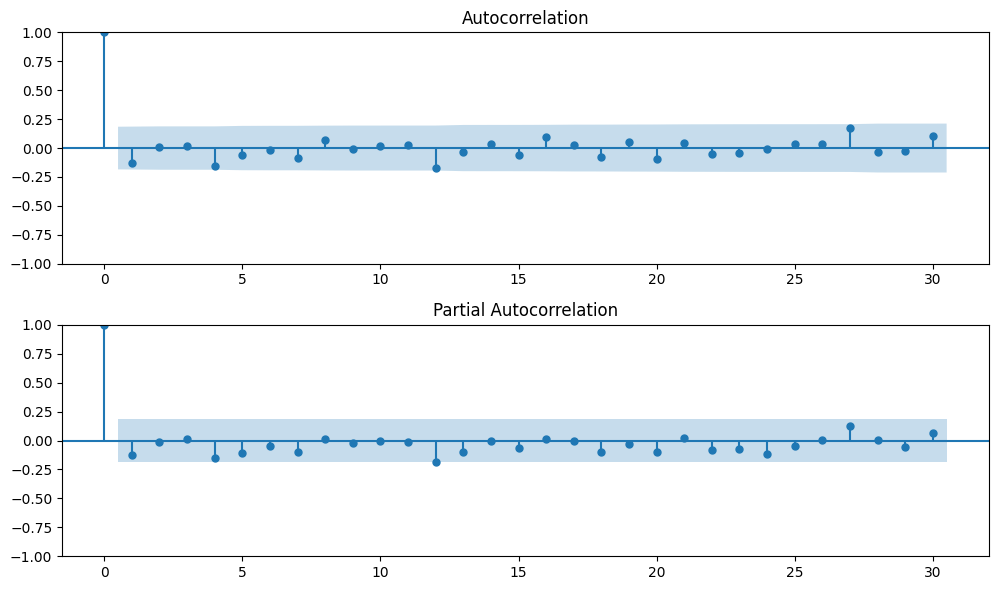
We plot the autocorrelation (ACF) and partial autocorrelation (PACF) of the differenced series to identify appropriate lag order for the AR model.

Output:

6. Splitting the dataset

We split the differenced data into training as 80% and testing as 20% to evaluate performance of the model.

7. Model Fitting

Using the lag order suggested by the PACF plot (example: p=13), we fit an AutoRegressive (AR) model on the training data.

8. Making Predictions

In this step we use the fitted AR model to produce both in‑sample “fitted” values on the training set and out‑of‑sample forecasts on the test set. We call the predict method of the AutoRegResults object, specifying

• start: the first timestamp at which to begin predicting.
• end: the last timestamp at which to predict.
• dynamic=False: means the model uses actual past values (not its own predictions) to make each forecast.

9. Evaluating the Model

We compute root‑mean‑square error (RMSE) and mean absolute error (MAE) on the differenced scale to quantify forecast accuracy.

Output:

1.3502853217579163
1.064373117847641

10. Invert Forecast to Original Scale

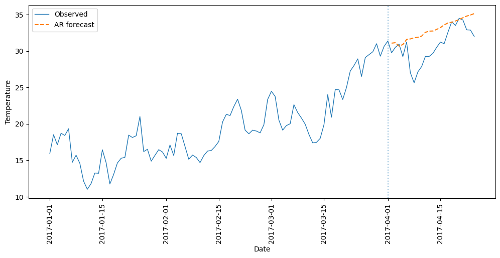
To compare your AR model’s output with actual temperatures you must turn the predicted daily changes () back into real temperature values (). We do this because the model was trained on the difference of the series (day‑to‑day changes) so its forecasts are in units of but we want forecasts in the original units (example: ) so we “undo” the differencing.

11. Potting the Results

Finally, we plot the full observed temperature series alongside the AR model forecast, marking the train/test split point.

Output:

Benefits and Drawbacks of Autoregressive Models

Benefits

• Simple and Easy to Use: AR models are straightforward to understand and implement.
• Interpretable: The coefficients show how past values influence future predictions.
• Good for Stationary Data: AR works well when the data has stable patterns over time.
• Fast and Efficient: They run quickly and are ideal for smaller datasets.
• Short-Term Pattern Detection: Effective at capturing recent trends and changes.

Drawbacks

• Requires Stationarity: Most real-world data needs preprocessing like differencing to meet this condition.
• Limited to Recent History: AR models can't capture long-term dependencies well.
• Choosing the Right Lag: Selecting too few or too many lag values can hurt performance.
• Sensitive to Noise: Random fluctuations can lead to inaccurate forecasts.
• Not Ideal for Long-Term Forecasting: Performance drops over longer prediction horizons.
• Data Quality Matters: Outliers or missing values can strongly affect accuracy.

Autoregressive models are tools for forecasting time series that show consistent patterns. In this article we applied an AR model to temperature to make predictions.

You can also read related articles:

• Time series analysis and forecasting.