Hazard Function - an overview

Hazard function estimates the probability that an item will fail during a specific time interval, based on its survival until the previous moment.

In simple terms, it reflects the risk of failure as time progresses, assuming that the item has survived up to the current time, and hazard function is denoted as ℎ(𝑡).

Hazard rate

Hazard rate is an important concept in reliability analysis and survival statistics, representing the rate at which an item or system fails at a given point in time, given that it has survived up to that point.

It provides insight into the likelihood of failure for an item of a particular age and is an essential component of the hazard function.

It can be represented as:

m

where:

• 𝑓(𝑡): The probability density function (PDF), representing the likelihood of the event occurring at time 𝑡,
• 𝑆(𝑡): The survival function, which measures the probability of "surviving" (not experiencing the event) up to time 𝑡.

Conditional Probability Interpretation

Alternatively, the hazard function can be expressed as:

This represents the instantaneous risk of the event occurring in a small interval, given survival up to time 𝑡.

Integrating ℎ(𝑡)allows recovery of the survival function:

Cumulative Hazard

The cumulative hazard function, 𝐻(𝑡), aggregates the risk over time:

Key Relationships: PDF, CDF, Survival, and Hazard

1. The Cumulative Distribution Function (CDF), 𝐹(𝑡), is related to 𝑆(𝑡) as:

2. The PDF, 𝑓(𝑡), is derived by differentiating 𝐹(𝑡):

3. The hazard function, in terms of 𝑓(𝑡) and 𝑆(𝑡), becomes:

Interpretation

• 𝑆(𝑡) decreases monotonically from 1 to 0 as time progresses.
• ℎ(𝑡) reflects the rate of change in risk over time.
• Hazard function that increases over time suggests that the risk of failure becomes greater as time progresses, while a decreasing hazard function suggests that the risk of failure reduces over time.

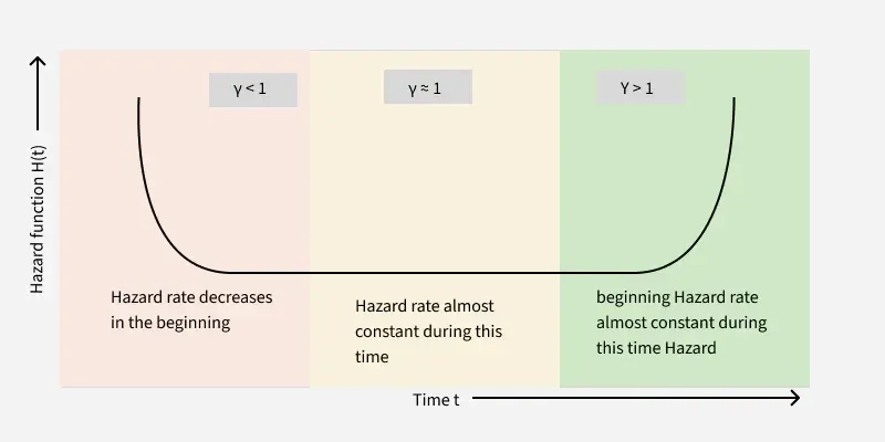
Different Types of Hazard Functions

The shape of a hazard function reveals crucial information about the process:

1. Constant Hazard: Exhibited by exponential distributions, where risk remains uniform over time. Example: Radioactive decay.
2. Increasing Hazard: Observed in aging systems where risk grows over time. Example: Mechanical wear and tear.
3. Decreasing Hazard: Seen in populations where risk diminishes as time progresses. Example: Infant mortality.
4. Non-Monotonic Hazard: Characterized by early failures followed by stable and increasing risk (e.g., the "bathtub curve").

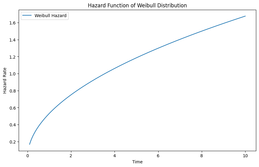
Weibull Distribution

A flexible model that encompasses increasing, constant, and decreasing hazards:

• If 𝛽<1: Decreasing hazard.
• If 𝛽=1: Constant hazard (exponential case).
• If 𝛽>1: Increasing hazard.

Weibull Hazard Function in Python

Output

The output represents hazard function of Weibull distribution, the shape of the curve is influenced by shape parameter and scale parameter of the Weibull distribution.

• Initial hazard rate is relatively low but increases steadily as time advances.
• As the time progresses, the risk of failure becomes more pronounced, indicating that the system's failure becomes more likely as it "ages."

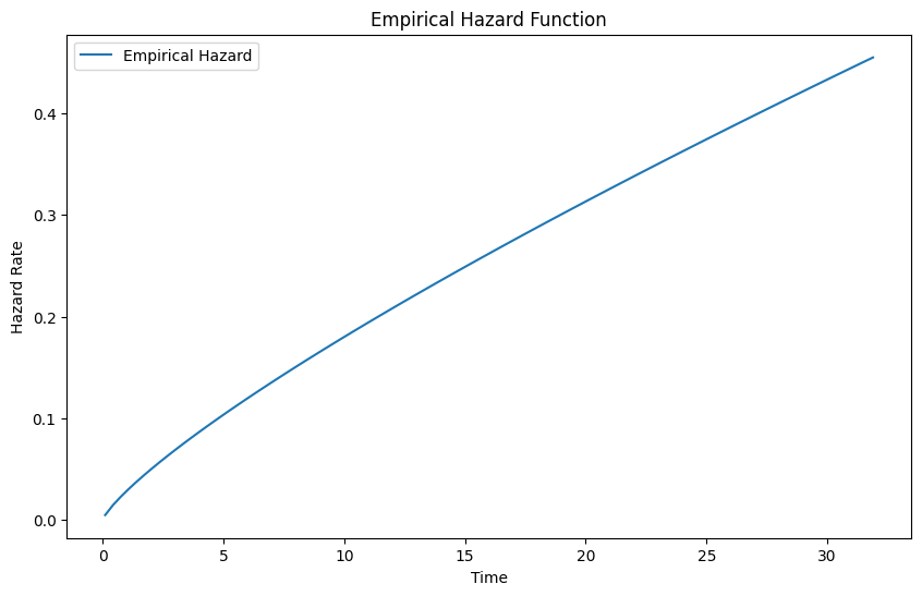
Practical Implementation: Case Study

Scenario: Analyzing survival rates of machinery in a factory. Using empirical data, we fit a Weibull distribution and estimate the hazard function.

Output:

• the hazard function is increasing, which reflects that the risk of failure grows over time.
• it is characteristic of systems that age or experience wear and tear.

Advanced Topics in Hazard Function Analysis

• Time-Varying Covariates: Exploring how covariates like age or stress levels influence hazard rates dynamically.
• Competing Risks: Analyzing scenarios where multiple event types compete (e.g., failure due to corrosion vs. fatigue).

Challenges and Limitations

• Assumptions of model parametricity may not always hold.
• Sparse data at tail ends can lead to unreliable hazard estimates.
• Non-parametric methods may require larger sample sizes.