Understanding Skewness and Kurtosis in Python

Understanding data distribution is essential in data analysis. Skewness helps identify whether data is symmetric or skewed, while kurtosis shows how heavy or light the tails are. In Python these measures can be computed quickly using built-in libraries.

Skewness

Skewness is a statistical measure used to describe the shape of a data distribution. It helps identify whether the distribution is symmetric or asymmetric, focusing on how data is spread around the central value rather than relying only on frequency distribution.

Types of Skewness

• Symmetrical Distribution: A distribution is called symmetrical if the left and right sides of the distribution are mirror images around the center point.
• Asymmetrical Distribution: A distribution is called asymmetrical if the left and right sides of the distribution are not identical around the center point.

Distribution Based on Skewness Value

• Skewness = 0: The distribution is normally distributed.
• Skewness > 0: The distribution has more weight in the left tail.
• Skewness < 0: The distribution has more weight in the right tail.

Kurtosis

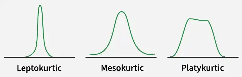
Kurtosis is a statistical measure that describes how strongly a distribution is affected by extreme values (outliers). It mainly reflects the heaviness of the tails compared to a normal distribution. While kurtosis is linked with the peak shape, it does not directly measure whether the distribution is sharp or flat at the center.

Types of Kurtosis

• Mesokurtic Distribution (Kurtosis = 3, Excess Kurtosis = 0): Represents a normal or near-normal distribution.
• Leptokurtic Distribution (Kurtosis > 3, Excess Kurtosis > 0): Has heavier tails than a normal distribution, meaning a higher chance of extreme values or outliers.
• Platykurtic Distribution (Kurtosis < 3, Excess Kurtosis < 0): Has lighter tails than a normal distribution, meaning fewer extreme values.

High Kurtosis Indicates

• Higher likelihood of extreme values
• More observations far from the mean
• Heavier distribution tails compared to normal

Low Kurtosis Indicates

• Lower likelihood of extreme values
• Fewer observations far from the mean
• Lighter distribution tails

How to Implement Skewness in Python

Step 1: Import Required Libraries

Here we import the necessary libraries for numerical computation, statistical analysis and visualization.

Step 2: Load and Prepare the Dataset

We use the built-in diamonds dataset from Seaborn and extract the price feature for analysis.

Step 3: Calculate Skewness Using SciPy

SciPy provides an inbuilt skew() function to compute skewness directly.

Syntax:

scipy.stats.skew(array, axis=0, bias=True)

Parameters:

• array: It represents the input array (or object) containing elements.
• axis: It signifies the axis along which we want to find the skewness value (By default axis = 0).
• bias = False: Calculations are corrected to statistical bias.

Return Type: Skewness value of the data set, along the axis.

Output:

Skewness using SciPy: 1.6183502776053016

A positive skewness value indicates that the distribution is right-skewed, meaning a longer tail on the right side.

Step 4: Pearson’s Second Coefficient of Skewness

Pearson’s Second Coefficient of Skewness measures skewness using the relationship between the mean, median and standard deviation. If the mean is greater than the median, the skewness value becomes positive, indicating a right-skewed distribution, while a negative value indicates left skewness.

Output:

Pearson's Second Skewness: 1.1518908587086387

Step 5: Visualizing Skewness

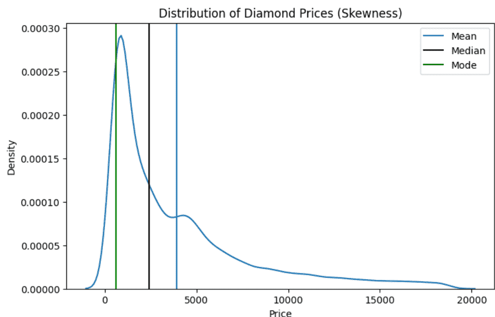
This step visualizes the distribution of diamond prices using a KDE plot and highlights the mean, median and mode with vertical lines to understand the skewness visually.

Output:

Since the mean lies to the right of the median and mode, the distribution is positively skewed, confirming the numerical skewness results.

How to Implement Kurtosis in Python

Step 1: Import Required Library

We import the kurtosis function from SciPy, which provides an inbuilt method to calculate kurtosis.

Step 2: Calculate Kurtosis Using SciPy

This step computes kurtosis using Fisher’s definition, where a normal distribution has a kurtosis value of 0.

Syntax:

scipy.stats.kurtosis(array, axis=0, fisher=True, bias=True)

Parameters:

• array: Input array or object having the elements.
• axis: It represents the axis along which the kurtosis value is to be measured. By default axis = 0.
• fisher = True: The fisher’s definition will be used (normal 0.0).
• fisher = False: The Pearson’s definition will be used (normal 3.0).
• Bias = True: Calculations are corrected for statistical bias, if set to False.

Return Type: Kurtosis value of the normal distribution for the data set.

Output:

Kurtosis using SciPy: 2.177382669056634

A positive kurtosis value indicates a leptokurtic distribution, meaning heavy tails and a higher presence of extreme values.

Step 3: Kurtosis for Multiple Numerical Features

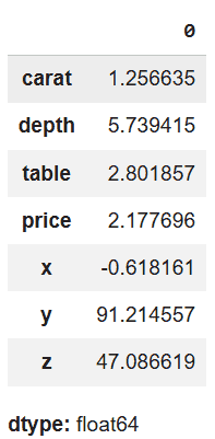
This step calculates kurtosis for all numeric columns to compare tail behavior across features.

Output:

Features with higher kurtosis values have heavier tails, indicating more outliers compared to features with lower kurtosis.

Step 4: Visualizing Kurtosis

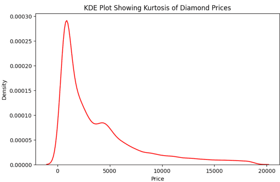
A KDE plot is used to observe the peak and tail behavior of the distribution.

Output:

The sharp peak and heavy tails in the plot indicate high kurtosis, supporting the numerical kurtosis values.

You can download full code from here