Singular Value Decomposition (SVD)

Singular Value Decomposition (SVD) is a factorization method in linear algebra that decomposes a matrix into three other matrices, providing a way to represent data in terms of its singular values.

SVD helps you split that table into three parts:

• U: This part tells you about the people (like their general preferences).
• Σ: This part shows how important each factor is (how much each rating matters).
• Vᵀ: This part tells you about the products (how similar they are to each other)

Lets understand this with help of an example: Suppose you have a small table of people’s ratings for two movies,

• SVD breaks this table into three smaller parts: one that shows people’s preferences, one that shows the importance of each movie, and one that shows how similar the movies are to each other
• Mathematically, the SVD of a matrix (of size ) is represented as:

Here:

• : An orthogonal matrix whose columns are the left singular vectors of .
• : A diagonal matrix containing the singular values of in descending order.
• : The transpose of an orthogonal matrix, where the columns are the right singular vectors of .

How to perform Singular Value Decomposition

To perform Singular Value Decomposition (SVD) for the matrix , let's break it down step by step.

Step 1: Compute

First, we need to calculate the matrix (where is the transpose of matrix ):

Now, compute :

Step 2: Find the Eigenvalues of

To find the eigenvalues of , we solve the characteristic equation:

Thus, the eigenvalues are and . These eigenvalues correspond to the singular values and , since the singular values are the square roots of the eigenvalues.

Step 3: Find the Right Singular Vectors (Eigenvectors of )

Next, we find the eigenvectors of for and .

For :
Solve :

Row-reduce this matrix to:

The eigenvector corresponding to is:

For :
Solve :
The eigenvector corresponding to is:

For the third eigenvector :
Since v₃​ must be perpendicular to and , we solve the system and , leading to:

Step 4: Compute the Left Singular Vectors (Matrix U)

To compute the left singular vectors U, we use the formula . This results in:

Step 5: Final SVD Equation

Finally, the Singular Value Decomposition of matrix is:

Where:

Thus, the SVD of matrix is:

This is the Result SVD matrix of matrix A.

Applications of Singular Value Decomposition (SVD)

1. Calculation of Pseudo-Inverse (Moore-Penrose Inverse)

• The pseudo-inverse is a generalization of the matrix inverse, applicable to non-invertible matrices like low-rank matrices. For an invertible matrix, it equals the inverse.
• Denoted as M^+ , it is calculated using the SVD , where and are orthogonal matrices of left and right singular vectors, and is a diagonal matrix of singular values.
• Pseudo-inverse formula: , where inverts non-zero singular values.

2. Solving a Set of Homogeneous Linear Equations

• For , if , use SVD to choose a column of associated with a zero singular value.
• If , solve by multiplying both sides by : .

3. Rank, Range, and Null Space

The rank, range, and null space of a matrix can be derived from its SVD.

• Rank: The rank of matrix is the number of non-zero singular values in .
• Range: The range of matrix is the span of the left singular vectors in matrix U corresponding to the non-zero singular values.
• Null Space: The null space of matrix is the span of the right singular vectors in matrix corresponding to the zero singular values.

4. Curve Fitting Problem

Singular Value Decomposition can be used to minimize the least square error in the curve fitting problem. By approximating the solution using the pseudo-inverse, we can find the best-fit curve to a given set of data points.

5. Applications in Digital Signal Processing (DSP) and Image Processing

• Digital Signal Processing: SVD can be used to analyze signals and filter noise.
• Image Processing: SVD is used for image compression and denoising. It helps in reducing the dimensionality of image data by preserving the most significant singular values and discarding the rest.

Implementation of Singular Value Decomposition (SVD)

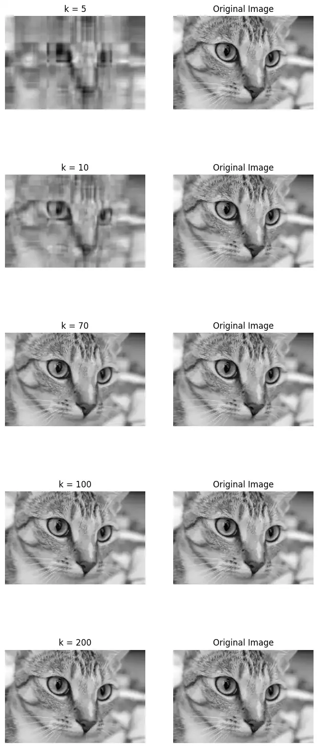
In this code, we will try to calculate the Singular value decomposition using Numpy and Scipy.  We will be calculating SVD, and also performing pseudo-inverse. In the end, we can apply SVD for compressing the image

Output:

[[ 3 3 2]
 [ 2 3 -2]]
---------------------------
U: [[-0.7815437 -0.6238505]
 [-0.6238505 0.7815437]]
---------------------------
Singular array [5.54801894 2.86696457]
---------------------------
V^{T} [[-0.64749817 -0.7599438 -0.05684667]
 [-0.10759258 0.16501062 -0.9804057 ]
 [-0.75443354 0.62869461 0.18860838]]
--------------------------
# Inverse 
array([[ 0.11462451, 0.04347826],
 [ 0.07114625, 0.13043478],
 [ 0.22134387, -0.26086957]])
---------------------------

The output consists of subplots showing the compressed image for different values of r (5, 10, 70, 100, 200), where r represents the number of singular values used in the approximation. As the value of r increases, the compressed image becomes closer to the original grayscale image of the cat, with smaller values of r leading to more blurred and blocky images, and larger values retaining more details.